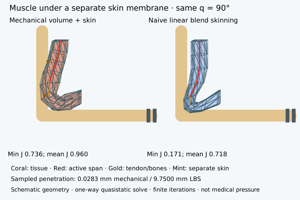
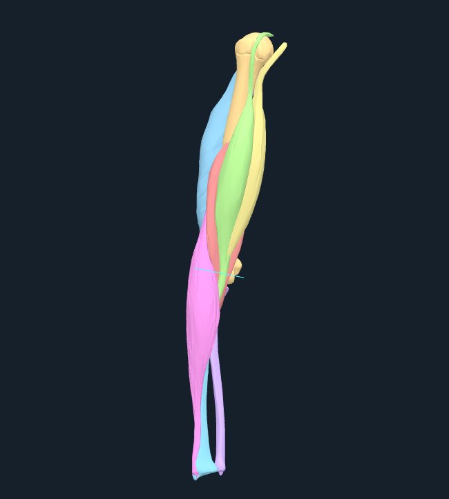
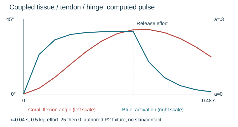
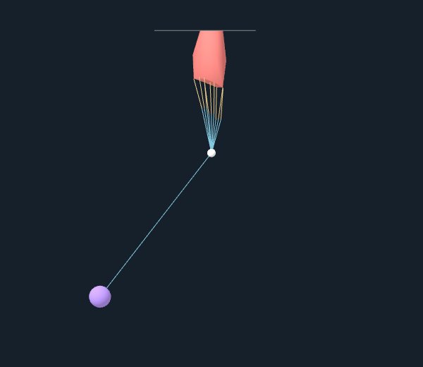
This mannequin starts in an authored neutral pose. Its graph and bound
surface describe geometry; they supply neither measured anatomy nor a
force law. Orbit the camera without changing the pose.
Observe The view changes while the prescribed pose
remains neutral. Force, pressure and contact response are not modeled.
Worked example · 2 / 3
Move a coordinate frame without deforming the body
Translate the root by 0.4 scene units in the poser’s horizontal
direction. Every local pose coordinate stays the same, so a moved
silhouette alone cannot establish tissue strain or mechanical work.
Observe The whole character moves together; the pose
graph and skin shape are unchanged. This is a prescribed placement, not
acceleration under force.
Worked example · 3 / 3
Change pose, then ask for the missing law
The existing hand-on-torso test prescribes a right-hand target and elbow
pole. Inverse kinematics chooses bone positions and geometric skinning
follows them. A tissue model would additionally need a material law,
boundaries, forces and convergence checks.
Observe The arm bends toward the torso. The pose does
not produce contact pressure or an equilibrium residual; these outputs
remain not modeled.
A body can look convincing while its forces are wrong. A model can
balance its forces while its surface looks wrong. Kenoma’s educational
book asks how to tell the difference, beginning with quantities that we
can calculate and inspect before adding anatomy. The intended reader is
a programmer, technical artist, or engineering student who wants to
connect geometry, mechanics, computation, and evidence.
This edition develops force, torque, energy, anatomical evidence, and
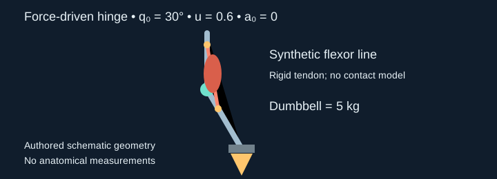
a force-driven schematic elbow with activation and a dumbbell load.
Seven original resettable 3D laboratories progress through compliant
tendon storage, a reduced continuum compression block, a worked
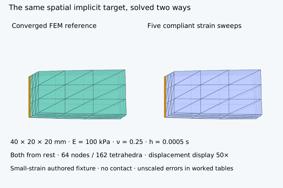
tetrahedral FEM/compliant-solver comparison, and a spatial
muscle-under-skin/contact strip at identical poses. An eighth,
worker-backed experiment jointly solves deforming tissue, distributed
tendons and a moving hinge. Its geometry is schematic; the requested
anatomical lifting capstone remains under development. A separate
evidence viewer contains ten actual atlas meshes, one recorded
normalized human trial, and six published model actuator parameter sets.
These are three independent evidence streams, not a calibrated person.
Three progressive property lessons additionally measure prescribed
tetrahedral deformation, compare isochoric volume with cross-section and
exterior area, and expose uneven axial strain in a nonuniform bar. A
fourth prescribed property lesson separates local from total volume
conservation under uneven finite stretch. Three further property lessons
add bulk/shear confinement, passive axial load/hold/release, and
force-driven unequal 3D blocks with individually preserved volume. The
printed edition contains the same explanations, static diagrams, data
figures, worked values and original numerical experiments. Clinical or
subject-specific prediction is not claimed or required to complete the
teaching examples.
The content is an educational extension. The
existing production plans in docs/plans/ remain separate. A
teaching experiment does not silently add a simulator requirement to the
Bevy MVP, change its canonical storage format, or establish a production
algorithm choice.
Reading path: measure first,
then add a law
Read force, torque and energy for the rigid-body
quantities and system boundary. Then use the three property
lessons in order: measure an imposed deformation; construct
prescribed volume preservation; calculate uneven strain under a reduced
axial law. Their worked examples introduce length, area, volume,
stretch, strain, force and stress before a contact or continuum solver
is needed. Continue with bulk/shear confinement,
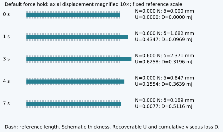
then load/hold/release to
distinguish recoverable storage from viscous loss in the passive axial
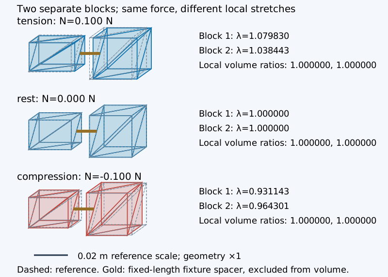
bar. Then compare unequal blocks under
one force, where a declared incompressible material law determines
the local stretches and current areas. This separate-block prerequisite
does not complete the requested connected continuous specimen with
varying cross section, coupled local axial/lateral deformation and
volume; that demonstration is not included or established in this
edition.
Next distinguish anatomical
evidence from teaching assumptions, and follow the actuator into elbow motion. The later tissue, tendon/compression and continuum chapters add
material energies, boundary conditions and force-driven deformation.
Prescribed constant volume is not a solved material response, and the
axial bar is not a full muscle. The fixed-field projection
interlude follows the spatial continuum comparison and precedes
interfaces and coupling. Its 27 exact finite weighted-vector statements
concern representation at one prescribed state. Spatial solver
comparisons and the anatomical research apparatus come after those
distinctions; their unfinished scope remains explicit.
Three different kinds of
evidence
A physical assumption describes the model: a
constant force, a perfectly rigid lever, or an ideal spring. A
numerical check compares the implemented arithmetic
with a reference or studies its error. A formal proof
establishes a precisely stated mathematical claim within its declared
domain. Each can be useful; none automatically supplies the other
two.
The 115 proof cards in this research edition are generated only after
checking fourteen source files with Lean 4.19.0:
Mechanics.lean, AnatomicalTransfer.lean,
CoupledMechanics.lean, AnatomicalArm.lean,
ContinuumProperties.lean,
MaterialResponse.lean,
MaterialResponseReal.lean, MechanicsReal.lean,
ActuatorConstitutiveReal.lean,
DissipativeBarReal.lean,
SerialSpecimenReal.lean, MixedLogVolume.lean,
NonuniformIsochoric.lean and
ArchitectureForce.lean. Thirty declarations use integer
domains and bundled Std, including five narrow material-response
contracts; eighty-five quantify reals with pinned mathlib v4.19.0. These
comprise four kinematic identities, five constrained specimen algebra
identities, three force/torque/power identities, eleven
activation/Gaussian/guarded-series results, eleven local
standard-linear-solid energy/relaxation results, twelve homogeneous
neo-Hookean serial-block identities, derivatives and ordering results,
27 finite weighted-vector projection results, six
declared-gradient/interval/algebraic-cell nonuniform-volume contracts
and six scalar architecture-force bookkeeping contracts. The actuator
results include real derivatives and conditional nonlinear root
existence/uniqueness; the compressible confinement specimen’s
constitutive derivatives and equilibrium obligations, continuous
actuator-mechanics work balances and numerical refinement remain
unfinished. Each card reports its exact theorem, assumptions, source
hash, implementation link and transitive axioms. The stated real results
do not establish floating-point equivalence, general force equilibrium,
anatomical validity or biological correctness. This distinction stays
visible beside each claim.
The new coupled fixture adds a deforming quadratic-tetrahedron block,
distributed tensile branches and an implicitly moving hinge whose tissue
torque comes from those branches. It is an intermediate engineering
experiment. The actual atlas arm, connected attachment patches and
interior-axis diagnostics are available separately for review; shared
anatomical tendons/aponeuroses and tissue contact are not yet accepted
or complete. The earlier schematic strip retains its declared one-way
coupling and is no longer presented as completion of the requested
anatomical capstone.
Coordinates and units
The original seven laboratories use a right-handed frame: x points
right, y points up, and z points out of the page. Laboratories 1–5 solve
planar motion or homogeneous block deformation and render them in a 3D
scene. Laboratories 6–7 add genuine spatial degrees of freedom; each
declares its constitutive and coupling limits. The coupled fixture
instead uses +Z downward, so its gravitational potential is −mgz. The
separate atlas assembly uses +X anatomical left, +Y posterior and +Z
superior. Each viewer identifies its own frame. The scene can be viewed
from the front or obliquely; changing the camera changes neither state
nor results. A 3D rendering does not turn planar equations into a
spatial biomechanical simulation.
Store physics in SI units and convert only at input and output. The
International System of Units names the metre, kilogram, and second;
force has unit newton, energy joule, and torque newton metre. Torque and
energy share dimensions but represent different quantities. We write
torque in N m to preserve that distinction. BIPM,
SI Brochure, §2.3.4
Quantity
Symbol
Unit
Meaning in the laboratories
Position
x
m
A coordinate in a specified frame
Time
t
s
Simulated time, distinct from wall-clock
playback
Mass
m
kg
Inertial mass, strictly positive in
controls
Force
F
N
A vector acting on a specified body
Torque
τ
N m
A moment about a specified origin and
axis
Energy
E
J
Scalar accounting for a defined
system
Spring stiffness
k
N/m
Force per extension in the ideal linear
spring
How to use a laboratory
Read the model label and the worked example first. Change one
control, predict a result, and inspect the numerical output before
interpreting the image. Step through time when needed; use Reset to
return all physics parameters and the camera to defaults. The
laboratories start paused and stop at a bounded step count. Laboratories
1–5 start a new experiment after a non-excitation parameter edit;
excitation edits in Laboratories 4–5 retain activation, velocity and
time. Laboratory 6 recomputes a static or single-step comparison rather
than integrating a trajectory. Laboratory 7 retains current activation,
time, pose, velocity and accumulated hinge work/dissipation across
parameter edits, then recomputes the spatial shape deterministically.
Its angle control explicitly sets pose with zero velocity and clears a
domain halt; entering prescribed hold stops motion at the current pose.
Reset and the 90° compression fixture deliberately initialize its state.
See each laboratory’s trace policy before comparing experiments. The
first four property lessons update static imposed geometry, an axial
calculation or a homogeneous material equilibrium without integrating
time. The fifth follows a finite SLS load/hold/unload/recovery protocol;
each parameter edit explicitly starts a new experiment and clears its
internal-state and energy history. The sixth property lesson recomputes
a static, force-driven two-block assembly without changing the requested
force; it exposes each finite root residual. The coupled fixture also
preserves its tissue coordinates, angle, velocity, activation and time
when effort or dumbbell mass changes. Its mass control records the
external energy added or removed with the mass; it does not restart the
trajectory.
Every scene has a text description and static illustration. If WebGL
is unavailable, the controls and numerical results still work. All seven
mechanics laboratories use original procedural schematic
teaching geometry: their cylinders, spheres, blocks, grids and
arrows are separate from anatomical measurements. The evidence viewer
instead shows actual licensed static atlas surfaces, with their source
labels, units and limitations. Neither the atlas nor the human-study
summaries calibrates the schematic actuator.
A useful question to carry
forward
Imagine a forearm holding a dumbbell. Ask: what system did we
isolate, what forces act on it, where do those forces act, and what
energy enters or leaves it? These questions remain useful whether the
next model is a rigid-body joint, a finite-element tissue mesh, or an
animation rig. A more detailed surface cannot rescue an unspecified
system boundary.
The property lessons use the same SI convention with prescribed
positive stretches or an explicitly reduced small-strain axial law. The
first four update a prescribed geometry or static equilibrium; the fifth
integrates an internal viscous strain under its stated axial law, and
the sixth solves two separate incompressible homogeneous blocks and
independently measures their 3D geometry. Independent geometric
measurements and midpoint-integration error remain visible; their exact
kinematic claims do not prove a constitutive law or qualify the
anatomical tissue envelope.
The architecture-force chapter and portable lab connect
reference/current area, nominal/Cauchy stress, projection, parallel
aggregation and series exchange. Every integrated artifact requires its
own complete-book proof receipts, browser/PDF checks and release
qualification. The historical nonuniform-volume total was 103 + 6 = 109;
this source registry adds six for 115. The preserved standalone
qualification does not establish complete-book proof closure, integrated
browser/PDF acceptance or anatomical calibration. All example counts,
areas, stresses and control ranges are authored.
Read the model before moving it
Every chapter now has an example in the shared Kenoma embedded GUI.
The label above each view distinguishes illustrative geometry,
prescribed kinematics, analytic bookkeeping, a numerical demonstration,
and recorded evidence. Orbiting a model does not increase its physical
dimension or validate its parameters. An algebraic statement can be
kernel-checked while its browser implementation, mesh approximation and
biological interpretation remain separate obligations.
The simple human poser is an independent artistic system: a graph,
generated surface and pose rig with gizmo controls and local SQLite
scene files. It has no tissue forces or contact response. Educational
model adapters share only presentation components with it. The research
apparatus retains its original laws, acceptance criteria and
failed-state evidence.
Checked cards show their claim, assumptions and limits immediately.
Expand a card for its exact statement, source and compilation receipt.
The complete Lean appendices are also collapsible on screen; the PDF
retains all statements and full sources. A GUI badge never substitutes
for the source-bound kernel receipt.
Interactive 3D · Coordinate and pose inspection
Illustrative geometry · related checked claims have separate
exact-domain scope
Move the root and hand targets; distinguish authored geometry from a
measured body.
No forces, contact, anatomical accuracy or clinical inference.
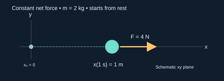
Start from rest with a constant 4 N horizontal net force on 2 kg. F/m
gives 2 m/s², so at 1 s the velocity is 2 m/s and the displacement is ½
× 2 × 1² = 1 m. The grey origin stays fixed; the arrow encodes force,
not velocity.
Observe Displacement = 1 m; velocity = 2 m/s. Work 4 ×
1 = 4 J equals kinetic energy ½ × 2 × 2² = 4 J.
Worked example · 2 / 4
Double time, quadruple distance
Keep the force and mass fixed and advance the analytic solution to 2 s.
Acceleration is unchanged. Velocity grows linearly with time, but
displacement grows with time squared. No time-stepping solver or
display-speed assumption enters this calculation.
Observe Displacement increases from 1 to 4 m, while
velocity increases from 2 to 4 m/s. Work and kinetic energy both become
16 J.
Worked example · 3 / 4
Double mass at the same time
Keep 4 N and 2 s but double the mass to 4 kg. The acceleration halves to
1 m/s². Both displacement and velocity halve relative to the previous
state; the change is caused by mass, not an animation setting.
Observe At 2 s, displacement = 2 m and velocity = 2
m/s. Work = kinetic energy = 8 J; the work-minus-kinetic residual is
zero.
Worked example · 4 / 4
Negative direction can mean positive work
Return to 2 kg and reverse the force. Acceleration, velocity and
displacement all point along negative x. The work is still positive
because force and displacement have the same sign: (−4 N)(−4 m) = 16 J.
Observe Displacement = −4 m and velocity = −4 m/s,
while work and kinetic energy are both +16 J. A negative force is not by
itself negative work.
A force is not a displacement instruction. For constant mass in an
inertial frame, the resultant external force determines acceleration.
Doubling force doubles acceleration; doubling mass halves it. Newton’s
second law and the separation of action-reaction pairs are presented in
Dourmashkin’s original course notes, §§7.3-7.4. Newton’s laws
Isolate the body before
adding arrows
Consider a small object translated horizontally by an actuator. The
schematic laboratory includes one constant horizontal net force. If we
imagined gravity and a support, their vertical balance would be an
additional assumption; this example simply solves the horizontal
component. Do not mistake its missing contact solver for evidence that a
support is physically correct.
For net force
,
mass
,
initial position
,
and initial velocity
:
Text equation: acceleration equals force divided by
mass. Velocity equals acceleration times elapsed time. Position equals
half acceleration times elapsed time squared, with both initial
conditions zero.
This is an analytic solution, so the force laboratory does not
accumulate time-integration error. JavaScript still evaluates
floating-point arithmetic. We compare selected outputs with exact worked
values using numerical tolerances; no theorem in this edition proves the
JavaScript implementation.
Laboratory 1 · Constant force
Analytic planar motion; constant net force; no contact or anatomy.
Static reference diagram. Step, Play or Pulse starts live 3D; if
unavailable, the display is explicitly numerical-only.
Reference at t = 1 s: m = 2 kg, F = 4 N, x = 1 m, v = 2 m/s. The
interactive starts at t = 0 s. Original schematic geometry.
A position marker moves along x. Position scale is fixed over the 0–2 s
trajectory for the selected mass and force; grid spacing is reported
below. Yellow force and violet velocity arrows use separate scales.
Values retain SI units. Axes: x right, y up, z out of the plane.
Worked example
Set mass to 2 kg and force to 4 N. The acceleration is 2 m/s². At 1 s
the position is 1 m and velocity 2 m/s. At 2 s the position is 4 m and
velocity 4 m/s. A negative force produces negative position and
velocity; the object accelerates along the negative x direction.
Try: keep force at 4 N, reset, and increase mass
from 2 to 4 kg. At the same simulated time the position is half as
large. Then set force to zero: position and velocity stay zero because
the initial velocity is zero. A zero force would preserve a nonzero
initial velocity in a different experiment.
Equal and
opposite forces belong to different bodies
If a tendon pulls a bone, the bone pulls back on the tendon. Those
two forces cancel in a combined bone-plus-tendon system. They do not
cancel on the isolated bone: only one member of that pair acts on it.
This is why a diagram with every arrow drawn on a single object can be
misleading.
For one scalar component, a pair
and
sums to zero. That identity is enough to check bookkeeping once we have
assumed an action-reaction pair. It does not prove that an actual
biological interface follows our chosen constitutive law.
The same assumed cancellation also holds for real force components,
without introducing an integer SI scale:
Work offers a second
calculation
A constant horizontal force does work
.
Starting from rest, the kinetic energy is
.
Substituting the analytic solution gives
in this ideal isolated horizontal model. For 4 N over 4 m, both are 16
J.
A negative force over a negative displacement also gives positive
work. Force direction alone does not determine work’s sign; the
force-displacement relation does. The next chapter keeps track of the
application point of that force, while the energy chapter studies what
happens when we replace analytic solutions with time steps.
Approximation boundary
This laboratory omits drag, friction, impacts, variable mass,
deformation, actuator limits, and all anatomy. Its moving sphere is a
marker for position, not a tissue particle whose radius or volume has
medical meaning. Positions beyond the viewing window are reported
numerically; the physical trajectory is not clamped to fit the
image.
Interactive 3D · Force, mass and displacement
Numerical demonstration · related checked claims have separate
exact-domain scope
Compare force, mass and elapsed time; check displacement and work
against kinetic energy.
Constant mass and constant horizontal net force; visual arrow lengths
are scaled.
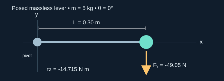
A 5 kg load exerts 49.05 N downward in the authored 9.81 m/s² field. The
0.30 m lever is horizontal, so τz = rx Fy = 0.30 × (−49.05) = −14.715 N
m. Positive z is counterclockwise viewed toward the origin.
Observe Moment arm = 0.30 m and torque = −14.715 N m. A
static pose would require an external +14.715 N m hold moment.
Worked example · 2 / 4
Separate lever length from moment arm
Rotate the same 0.30 m lever to 60°. Its horizontal offset is 0.30 cos
60° = 0.15 m, even though its length is unchanged. Gravity acts along
the grey vertical line; the orange horizontal segment is the
perpendicular offset.
Observe Moment arm = 0.15 m and torque = −7.3575 N m:
exactly half the horizontal-case magnitude within floating-point
precision.
Worked example · 3 / 4
Put gravity through the pivot
At 90°, gravity’s line of action passes through the pivot. The force is
still 49.05 N, but its perpendicular offset is zero. This is a posed
geometric calculation, not a prediction that the lever stays there
without supports.
Observe Torque is approximately −9.01 × 10⁻¹⁶ N m and
moment arm approximately 1.84 × 10⁻¹⁷ m: numerical zero, not a small
physical moment.
Worked example · 4 / 4
Cross the pivot and reverse the moment
At 120° the load is left of the pivot: rx = −0.15 m. Multiplying this
negative offset by the downward force gives a positive moment. The
unsigned moment-arm magnitude alone cannot tell you the rotation
direction.
Observe Moment-arm magnitude remains 0.15 m, but torque
is now +7.3575 N m. The required static hold moment reverses to −7.3575
N m.
A force that passes through a pivot produces no moment about that
pivot. The same force applied farther from the pivot can produce a
larger moment. The laboratory introduces the moment of a force about a
chosen origin; the definitions and axis convention are verified against
Dourmashkin’s rotational-dynamics notes, §17.1. Rotational dynamics
A planar cross product
Let
point from the pivot to the application point, and
be the force on the lever. The component along z is:
Text equation: torque around z equals x position
times y force minus y position times x force. Positive torque is
counterclockwise when viewed from positive z toward the origin.
In the schematic example a massless rigid lever of length
supports a point load of mass
at its tip. The angle
is measured counterclockwise from the horizontal, not from a clinical
elbow coordinate convention. Uniform gravity is
,
with illustrative
m/s². Therefore:
This is a posed lever. The slider prescribes its angle; no active
muscle, torque controller, angular acceleration, or joint-contact force
maintains the pose. A physical static hold would require an opposing
moment supplied by some actuator and appropriate support forces.
Laboratory 2 · Force and lever arm
Prescribed pose; massless rigid lever; point load; uniform illustrative
gravity.
Static reference diagram. Start interactive 3D to view current results;
numerical controls also work without 3D.
Default: m = 5 kg, L = 0.30 m, θ = 0°. Torque about z is -14.715 N m.
Original schematic geometry; no anatomical measurements.
A rigid bar extends from a fixed pivot to a load. The yellow arrow
points downward. The white projection marks the horizontal distance to
the gravity line. This is a posed lever, not an active arm. Axes: x
right, y up, z out of the plane.
Worked values and the moment
arm
At
kg,
m, and
°,
gravity is 49.05 N downward and torque is -14.715 N m. At 90° the line
of gravity passes through the pivot and the moment is zero within
floating-point tolerance. At 120° the torque becomes positive because
the load lies on the other side of the pivot’s vertical line.
The perpendicular moment-arm magnitude is
.
It is not generally the lever length. Its magnitude tells us how
strongly gravity acts about this pivot, while the cross product retains
direction.
Try: compare 0°, 60°, and 90°. Predict the torque
ratio before moving the slider. At 60° the torque magnitude is half the
horizontal value. Move from 89° to 91° and watch the sign change.
The exact worked arithmetic can be represented by 300 mm and -49050
mN. Multiplying those scales gives
N m per integer product unit. The following theorem checks the integer
cross product; division by one million to obtain SI torque is an
explicitly stated interpretation.
Combining forces
Two forces at the same point contribute torques that add. We can
either add their force vectors first or add the two moments. The
identity is useful when assembling muscle and external-load
contributions around a joint.
For the real quantities in the stated cross product, the
corresponding identity is checked separately:
It is unsafe to add torques computed around different origins without
transforming them. If the new origin is at
relative to the old one, the position becomes
,
and:
Internal forces and couples
Equal and opposite forces can have zero resultant force and a nonzero
resultant torque. Think of two forces acting along different parallel
lines: they form a couple. Force cancellation alone is not enough to
infer moment cancellation.
For a central pair between positions A and B, let the force at A be
and the force at B its negative. Their summed moment vanishes because
both forces act along the joining line. The theorem checks this
specifically for planar integer coordinates and integer k.
This assumption should be inspected before applying it to a tissue
model. A model that exchanges angular momentum through distributed
stress or explicit bending moments needs the corresponding moment
balance, not a point-force argument with missing terms.
Connecting torque to energy
The point load has gravitational potential
relative to its horizontal position. Differentiating with respect to
angle in radians gives
.
A finite-difference numerical test checks this relation for the
implemented lever. It does not establish a floating-point theorem. This
independent calculation is valuable because it can reveal a sign
convention or degree/radian conversion error.
Interactive 3D · Moment arm in three dimensions
Numerical demonstration · related checked claims have separate
exact-domain scope
Change the planar lever angle and inspect the moment vector.
Planar mechanics rendered in 3D; no joint or anatomical inference.
Use the same 1 kg, 40 N/m spring starting at x = 0.20 m and v = 0. At h
= 0.05 s, explicit Euler multiplies energy by 1 + 40h² = 1.1 each step.
After 40 steps, t = 2 s and E = 0.8 × 1.1⁴⁰.
Observe Energy grows to 36.2074 J, a maximum deviation
of 4425.93%. Position is 1.27918 m, versus analytic 0.199316 m at the
same 2 s.
Worked example · 2 / 4
Change the update, preserve the experiment
Keep the initial state, step size and 2 s endpoint. Updating velocity
before position changes the numerical method. Its endpoint energy looks
much closer, but inspect the maximum over every completed step rather
than trusting a single snapshot.
Observe Final energy is 0.766327 J, while maximum
energy deviation is 18.7744%. Absolute position error is 0.00550736 m.
Bounded-looking motion does not imply exact conservation.
Worked example · 3 / 4
Use both endpoint accelerations
Velocity Verlet uses old and new acceleration. The same 40 steps reach
the same physical time. At this endpoint the energy happens to lie very
near 0.8 J; the maximum over all samples prevents that phase coincidence
from hiding error.
Observe Final energy is 0.799632 J, but maximum energy
deviation is 2.49928%. Position error is 0.00116381 m. These are
measured numerical errors, not a conservation proof.
Worked example · 4 / 4
Refine at equal elapsed time
Reduce h fivefold and use five times as many steps so the endpoint
remains 2 s. Comparing equal step counts here would compare different
experiments. The finer run uses the same physical model and no retuned
constants.
Observe Maximum energy deviation falls to 0.0999895%
and endpoint position error to 0.0000353055 m. Both improve in this
experiment; this does not establish a universal error bound.
Energy accounting can expose a trajectory that looks smooth while
gaining energy from its numerical update. The definitions of kinetic
energy and work are verified against Dourmashkin’s notes, §§13.2-13.6.
Energy and work The numerical experiment
below is original code and analysis in this repository; it is a
synthetic oscillator experiment, not new biological data.
An ideal
oscillator with a reference solution
A mass attached to a linear spring has extension x and velocity v.
There is no damping, gravity, contact, or active energy input. Its
equation and total mechanical energy are:
Text equation: mass times acceleration equals
negative stiffness times extension. Energy equals half mass times
velocity squared plus half stiffness times extension squared.
The default parameters are
kg,
N/m,
m, and
m/s. Initial energy is 0.80 J. The angular frequency is
,
and the reference trajectory is
,
.
Laboratory 3 · Numerical energy
Ideal undamped linear spring; fixed physics steps; 12 simulated seconds
per trajectory; 120–2,400 fixed steps for the supported h.
Static reference diagram. Step, Play or Pulse starts live 3D; if
unavailable, the display is explicitly numerical-only.
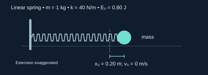
Initial state: m = 1 kg, k = 40 N/m, x = 0.20 m, v = 0 m/s, E = 0.80 J.
Default symplectic Euler step h = 0.02 s. Original schematic geometry.
A spring connects a wall to a mass marker. Extension is visually
exaggerated and fitted to the view. The energy chart shows a solid
numerical trace and a dashed initial-energy reference. Read numeric
values when the chart rescales. Axes: x right, y up, z out of the plane.
Three ways to take a step
Let h be a positive time step in seconds, and
.
Explicit Euler updates both values from the old
state:
Symplectic Euler updates velocity before
position:
Velocity Verlet includes the new acceleration:
The methods are implemented separately from rendering. Playback
advances fixed simulation steps and reports their index and elapsed
time; it never inserts the browser’s frame duration into the physics
formula. Play advances approximately one simulated second per wall-clock
second. Run to 12 s finishes the current trajectory in
bounded frame batches; either running mode can be paused and resumed.
Each supported h reaches the same 12-second endpoint (120–2,400 steps),
and every physics sample is retained even when the display redraws only
once per frame. The readout reports completed/total steps,
elapsed/target time, the maximum energy deviation over all samples and
the current position error against the analytic reference. Download
trace preserves all samples and these measurements. A parameter change
starts a new trajectory. Reset reproduces the same sequence for a given
method and step size.
Why explicit Euler gains
energy
Substitute the explicit update into the quadratic energy and expand.
The mixed terms cancel, leaving:
For positive k, m, and h, every nonzero-energy step multiplies energy
by a factor greater than one. Making h smaller delays the growth; it
does not produce bounded energy over arbitrarily long time with fixed h.
This is a paper-and-pencil derivation for the ideal oscillator. No Lean
theorem in this edition checks that integrator identity.
For the other two methods, the linear oscillator’s usual bounded
regime is
.
Even inside that regime, neither method preserves the exact physical
energy at every step. The observed energy oscillates, and phase error
accumulates. A stable picture and an accurate time history are different
checks.
Original reproducible
experiment
Run each method with the same initial conditions over 12 simulated
seconds. Compare h = 0.01, 0.02, and 0.05 s, measuring the maximum
absolute relative energy deviation over all sampled
steps and the final absolute position error against the analytic
reference. No wall-clock speed claim is made. The table below is
generated by executing web/mechanics.mjs, the same pure
physics module used by the browser.
Method
h (s)
Steps
Max relative energy deviation (%)
Final position error (m)
explicit
0.01
1200
1.194e+04
1.849
explicit
0.02
600
1.368e+06
23.11
explicit
0.05
240
8.595e+11
5848
symplectic
0.01
1200
3.266
0.004304
symplectic
0.02
600
6.752
0.01165
symplectic
0.05
240
18.78
0.0622
verlet
0.01
1200
0.09999
0.00122
verlet
0.02
600
0.4
0.005052
verlet
0.05
240
2.5
0.03887
The final position error can be small by phase coincidence; it should
not be used alone to select a method. The energy maximum shows explicit
Euler’s growth even when a snapshot happens to cross the reference.
Symplectic Euler has a larger oscillating energy deviation than Verlet
for these settings. Both still require refinement studies for any
intended application.
Try: reset with explicit Euler and h = 0.05 s. Step,
play or run to 12 s to see the energy increase. Reset with Verlet at the
same h. Compare numeric energy with the dashed 0.80 J reference, then
halve h and compare again. The plotted vertical range adapts to the
computed energy; read its numeric maximum so that rescaling cannot
disguise instability.
A modest formal claim
With a nonnegative exact integer mass, the numerator
is nonnegative. With positive unit scales and the factor one half, it
corresponds to nonnegative kinetic energy. That claim says nothing about
conserving energy from one step to the next.
Approximation boundary
The spring is linear at all extensions, including compression, and
has no tensile-only constraint. It is therefore not a tendon model. An
active muscle adds energy through a contraction law; a dissipative
tissue removes energy; contact may exchange or dissipate energy. Before
interpreting their energy residuals, include those terms and define the
model’s system boundary.
Before adding those material mechanisms, continue to the three
property lessons. They measure an imposed shape, construct
constant-volume kinematics, and calculate nonuniform strain with one
declared axial law. This separates geometric observations from the force
and energy models that will later produce them.
Interactive 3D · Oscillator state and energy
Numerical demonstration · related checked claims have separate
exact-domain scope
Compare integrators at equal elapsed time, then refine the step size and
inspect maximum sampled energy error.
One-dimensional oscillator rendered in 3D; numerical drift is not a
checked conservation theorem.
Unit stretches and zero shear prescribe the identity map. Compare the
determinant with volume measured independently from the closed boundary
triangles.
Observe Both volume ratios are 1; Green strain is zero
up to floating-point roundoff. The coincident surfaces are expected.
Worked example · 2 / 4
Lengthen one direction
Only the X direction is stretched. The transverse stretches stay 1, so
det F = 1.2 × 1 × 1 = 1.2.
Observe Both volume ratios become 1.2. Green strain
norm is 0.22; these are imposed geometric changes, not a force response.
Worked example · 3 / 4
Change shape while keeping volume
Restore axial stretch to 1 and impose shear 0.25. The triangular
deformation matrix still has unit determinant, but its reference
Y-directed edge becomes longer.
Observe J stays 1 while Green strain norm is about
0.179518 and Y-line stretch is about 1.03078. Constant volume does not
mean zero strain.
Worked example · 4 / 4
Rotate without adding strain
Rotate the same sheared geometry by 90 degrees. Rigid rotation changes
world-space positions but preserves edge lengths and F-transpose F.
Observe The geometry rotates; J, Green strain norm and
Y-line stretch match the previous step. No material law or equilibrium
has been introduced.
These progressive property lessons separate geometry, constitutive
response and equilibrium. A shape that keeps its total volume can still
have uneven local compression; a shape that looks muscular has not
thereby passed a mechanical test. The anatomical capstone retains its
failed cases and its force and geometry gates.
Start here after force, torque and energy. First ask
what changed in the shape? Then impose a simple volume
relation. Finally introduce one axial force law to ask why different
sections strain differently. No contact solver, anatomical mesh or
finite-element assembly is needed for these three lessons. The later material chapter
adds energy, stress and equilibrium in three dimensions.
Quantity
Units
How to read it here
Reference/current positions
;
length
m
Positions before/after an imposed change;
distance along the bar
Cross-section
;
boundary volume
m²; m³
Area across the axial direction; volume
enclosed by oriented faces
Stretch
;
volume ratio
dimensionless
Current/reference length or volume; one
means unchanged
Deformation gradient
;
strain
dimensionless
Local shape map; measures of deformation,
not forces
Axial resultant
N
Total tensile force through a section, not
stress at a point
Modulus
;
active-stress offset
Pa = N/m²
Parameters of the declared axial material
law
Activation coefficient
dimensionless, 0–1
Static multiplier of the authored stress
offset, not an integrated activation trajectory
Compliance
m/N
Extension per applied force in the passive
bar
The symbol
below is a deformation matrix, not the force vector of Laboratory 1. The
bar’s
is a modulus, not energy in joules;
denotes Green strain. Stretches and strains have no units: stretch 1.2
means 20% longer, while axial strain 0.01 means 1% extension in the
small-strain bar. These static property lessons do not advance time,
integrate activation or calculate metabolic energy.
1. Measure a prescribed
deformation
Question: if we move the vertices ourselves, how do
we measure stretch, shear and volume change? The reference tetrahedron
has four vertices; its three edges from vertex zero are stored as the
columns of
.
The current edges form
.
Multiplying by
removes the original edge scale, so
maps a small reference edge to its current edge. You can begin with the
numerical stretch and volume readouts before working through this matrix
notation.
For reference vertices
and current vertices
,
each in metres, construct edge matrices
and
.
A nondegenerate, positively oriented reference is required. The affine
deformation gradient, local volume ratio and Green strain are
The controls impose
with
,
then add a common translation:
.
Column vectors are used;
acts first, the rigid rotation second. The off-diagonal coefficient
is entered directly; this is not a shear matrix multiplied after a
separately defined stretch. The diagonal coefficients are not all
material-line stretches when shear is present. The reference X, Y and Z
line stretches are
,
and
,
respectively; the browser independently measures them from the
transformed edges. Rotation and translation leave those line lengths
unchanged.
Translation cancels from the edges. A rigid rotation has
;
simple shear can have
while
.
Volume preservation does not mean absence of strain.
The independent measurement uses the oriented boundary triangles. For
any common origin
,
with outward face ordering,
The browser computes this triangle sum without calling the
determinant helper. It reports
,
in dimensionless units, rather than assuming agreement. Negative signed
volume or nonpositive
rejects the candidate and retains the last valid displayed state. This
four-node affine test does not certify curved P2 elements or a whole
moving tissue envelope.
Property lab 1 · Measure deformation
Declared reduced fixture; SI units; scope and assumptions in the
adjacent derivation.
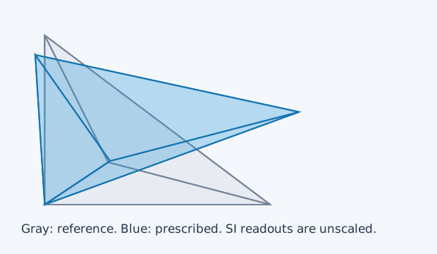
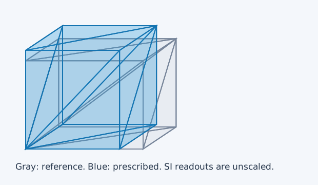
Authored 80 × 60 × 50 mm reference. Gray is reference; blue is
prescribed geometry. This lesson imposes kinematics and does not solve
force equilibrium.
Authored 80 × 60 × 50 mm reference. Gray is reference; blue is
prescribed geometry. This lesson imposes kinematics and does not solve
force equilibrium.
Try and predict. Set all three diagonal coefficients
to 1, shear and rotation to 0. The measured
and boundary-volume ratio should both be 1, and Green strain should be
zero. Change only translation X to 30 mm: it moves the tetrahedron but
changes neither measurement. Next set axial stretch to 1.2: expect
.
Restore unit diagonal coefficients and set shear to 0.25: volume stays
the same, but Green strain is nonzero. Rotation alone also keeps volume
and strain unchanged; the components of
can still change.
The controls prescribe the vertices. This lab measures
,
,
Green strain and an independent boundary volume; it solves no forces,
material energy, contact or equilibrium. A valid positive volume is a
geometry check, not evidence of a realistic muscle response.
2. Exact isochoric kinematics
Question: what lateral change would keep a
rectangular block’s volume exactly fixed while its axial length changes?
Isochoric means constant volume. Here we impose the answer; no
pressure or material stiffness chooses it.
Prescribe
with positive dimensionless stretches. Then
.
In the isochoric construction
,
so
in exact real arithmetic. The interactive controls also allow
independent stretches, which need not preserve volume. This is a
kinematic construction, not a minimization or a muscle contraction
law.
For the rectangular reference,
,
and
.
Cross-section area is the area normal to the axial direction, measured
from two transverse edges. Exterior area is the sum of all
boundary-triangle areas. They have the same units, square metres, but
different mechanical meanings. Neither is automatically physiological
cross-sectional area (PCSA). The independent boundary-volume measurement
remains visible when the isochoric toggle is selected.
Property lab 2 · Volume and cross-section
Declared reduced fixture; SI units; scope and assumptions in the
adjacent derivation.
Authored 80 × 60 × 50 mm reference. Gray is reference; blue is
prescribed geometry. This lesson imposes kinematics and does not solve
force equilibrium.
Authored 80 × 60 × 50 mm reference. Gray is reference; blue is
prescribed geometry. This lesson imposes kinematics and does not solve
force equilibrium.
Try and predict. At axial stretch
,
the 0.08 m reference length becomes 0.064 m. The imposed lateral stretch
is
,
so the reference cross-section 0.003 m² grows to 0.00375 m². Their
product remains 0.00024 m³. Switch to independent stretches and set
:
the same shortening now gives
.
Read cross-section area and exterior area separately; they need not
change by the same factor.
This volume-preserving motion is prescribed
kinematics, not material-driven volume redistribution. The
free-side compression example in Laboratory 5 later determines lateral
stretch from a material law and boundary conditions, rather than
imposing this square-root relation. Neither lesson specifies a complete
deforming muscle.
3. Nonuniform
cross-section: a reduced axial oracle
Question: can one constant tensile force produce
different strain along a bar? Here shape is no longer prescribed at
every section. We assume a one-dimensional material law and axial
balance, then calculate strain. Positive strain is extension; negative
strain is compression. The coordinate
runs along the reference bar;
is axial stress in pascals. Larger area or modulus reduces passive
strain at the same force.
Take a small-strain bar with length
in metres, positive area
in square metres, constant modulus
in pascals, no distributed axial load, and a tensile-positive resultant
in newtons. Force balance gives
.
The passive law gives
,
so
A1 is the reference area at s=0 and A2=rA1 is the end area at s=L.
The ratio permits either direction of taper: for r<1, A2 is the
narrow end; for r>1, A1 is the narrow end. The readout derives
narrow/wide areas from the selected geometry.
For linear area taper
,
the exact compliance is
,
with limit
at
.
Numerical midpoint integration is compared with that analytic integral.
Linear area taper is a separate geometric assumption from a radius
taper. The exterior surface influences surface traction and contact; it
does not replace
in this axial law.
Add a separately declared uniform active-stress offset
,
still under this reduced small-strain law:
.
With both ends fixed,
determines the constant
.
Two equal-length segments with
and
give
,
narrow strain
and wide strain
.
Local extension and compression coexist even though total length is
fixed. This offset model has no force–length/velocity dependence,
transverse equilibrium, pennation, ECM, fluid or anatomical calibration;
it is not a complete active muscle model.
Property lab 3 · Uneven axial strain
Declared reduced fixture; SI units; scope and assumptions in the
adjacent derivation.
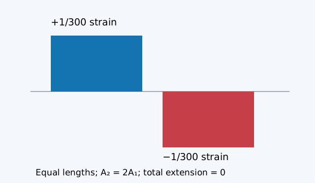
Small-strain constant-modulus bar; no distributed axial load. Strain by
axial position, with blue extension and red compression. Area controls
an axial resultant, not a complete muscle law.
Small-strain constant-modulus bar; no distributed axial load. Strain by
axial position, with blue extension and red compression. Area controls
an axial resultant, not a complete muscle law.
Try and predict. In passive mode, keep the default
geometry and modulus and change force from 0.3 to 0.6 N: every strain
and the total extension double. Doubling the modulus instead halves
them. In active fixed-end mode, choose two equal-length segments and
keep area ratio 2, activation 1 and active stress 1,000 Pa at modulus
100,000 Pa. The narrow section extends by
and the wide section compresses by
,
while their total length change is zero. Passive force is disabled in
that mode because the fixed-end compatibility determines the reaction;
active controls are disabled in passive mode.
This bar solves an axial resultant and axial strain under its stated
assumptions. It does not determine lateral stretch, cross-section
evolution, transverse stress, contact, three-dimensional fibre
aggregation or muscle shape. The area profile is an input; neither zero
net extension nor the active-stress offset supplies the missing
transverse equilibrium. Refining midpoint cells improves the integral of
this same reduced law, not its biological scope.
The illustrative 5% small-strain warning uses the true endpoint
extrema of this monotone positive-area law, independent of midpoint
display resolution. It is a warning about this approximation, not
material validation.
The executable oracle is the
tapered-bar module. Tests check the logarithmic integral, refinement
and the two-segment fixed-end case. Its scope is numerical evidence for
this declared reduced law; the kinematic Lean claims above do not prove
its mechanics.
Continue with anatomical evidence
before assigning these quantities to a named muscle. When you reach tissue and rendered skin, reuse the
measurements above while adding a material law and boundary forces. The
next material-response
lesson adds bulk/shear and unilateral confinement controls. Load/hold/release now adds a
bounded passive axial SLS lesson. The
two-block specimen then solves unequal 3D stretches and current
areas under one force, with an explicit incompressible material
constraint. Measured fibre-to-muscle aggregation and
force–length/velocity lessons remain pending, as recorded in the coverage chapter.
What the exact claims cover
The freshly checked real-number proof bundle establishes edge
translation invariance, determinant composition, the actual diagonal
determinant and the positive square-root isochoric construction. The
four claims above are compiled from their displayed real definitions
against pinned mathlib. The edge and matrix identities do not prove the
oriented boundary-triangle oracle, and the isochoric identity does not
prove a free-side material equilibrium. Separate numerical and browser
tests cover the implemented controls and boundary measurements. Neither
class of test validates measured biological parameters or resolves the
capstone’s local compression and full nodal stationarity failures.
Interactive 3D · Reference and deformed tetrahedron
Prescribed kinematics · related checked claims have separate
exact-domain scope
Change axial stretch and shear; compare determinant with
triangle-measured volume.
Prescribed affine map, not force equilibrium or tissue response.
Mean stretch is 1 and the uneven-stretch amplitude is zero. Local
compensation is then the identity everywhere.
Observe Local J and both total volume ratios are 1 up
to triangle-sum roundoff.
Worked example · 2 / 4
Let local volume changes cancel
The endpoint axial stretches are 0.6 and 1.4. Without transverse
compensation, J equals the local axial stretch; the average remains 1.
Observe Total continuum volume remains 1 while local J
spans 0.6–1.4. A correct global volume cannot establish local
incompressibility.
Worked example · 3 / 4
Compensate every material section
Set transverse stretch to 1/sqrt(lambda) at each section. This makes the
exact map locally isochoric, but eight straight mesh cells only
approximate its curved boundary.
Observe Local J is 1 throughout. The measured mesh
ratio is about 1.00248, an excess of 0.00247970 rather than an exact
mesh-volume guarantee.
Worked example · 4 / 4
Refine the geometric measurement
Keep the same continuum map and increase only longitudinal cells from 8
to 128. This tests the straight-boundary approximation, not a different
material.
Observe Mesh-volume error falls to about 0.00000968811.
The exact local and continuum volume ratios remain 1; the nonzero
numerical discrepancy stays visible.
The previous property lesson measured homogeneous deformations. Now
prescribe a smooth deformation along one reference prism: neighbouring
material sections can stretch differently while each point preserves its
volume. This is an imposed geometric map, with no force balance, passive
material response, activation or anatomical prediction. It is a
different construction from the later serial specimen, whose two
separate homogeneous blocks are joined by a spacer.
A complete gradient, including
shear
Let the material coordinate satisfy
,
with
,
mean stretch
and dimensionless uneven-stretch amplitude
.
The reference section is a regular 16-sided polygon of circumradius 15
mm; the reference length is 120 mm. Define
The transverse coordinates are
and
,
with
under local compensation and
otherwise. Differentiating the map gives
The actual stretch gradient is
,
with units of inverse length. Under compensation,
.
The off-axis terms describe shear; dropping them would misstate the
gradient even though its determinant would agree. The displayed
engineering strain
refers to the centerline, not every surface fibre.
Positivity makes the axial map strictly increasing, and positive
transverse scaling makes the map injective. The ordinary
change-of-variables argument then gives continuum volume conservation
when
.
These differentiation, injectivity and integration arguments are
separately audited mathematical reasoning. The Lean declarations below
prove properties of the declared matrix, positive
stretch on the stated interval and an algebraic straight-cell error
formula; they do not formally prove those analytic arguments or the mesh
implementation.
Compare local and total
conservation
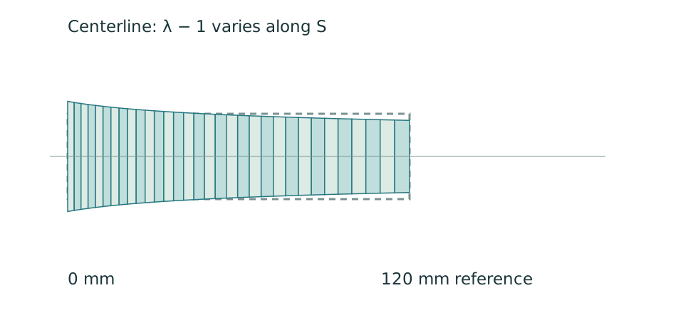
Default prescribed geometry: m = 1, a = 0.4, 32 axial cells, 16 polygon
sides and local radial compensation. Teal strips share the full mesh
vertices. Fixed scale: 4 SVG units/mm; reference length 120 mm,
circumradius 15 mm.
Open the interactive
local-volume lab. Change mean stretch, uneven-stretch amplitude,
mesh cells and local compensation; reset returns to the declared
reference. The full six-contract inventory, complete Lean source and
independent audit downloads are bundled with the lab.
At
,
,
local compensation gives endpoint stretches 0.6 and 1.4, while
throughout. Disable compensation: the total continuum volume ratio still
equals one, but the local Jacobian ranges from 0.6 to 1.4. Expansion and
contraction cancel globally. Total volume alone cannot establish local
incompressibility.
The closed three-dimensional boundary mesh and its displayed
longitudinal section use the same vertices and fixed millimetre scale.
Signed boundary-triangle volumes are independently compared with
regular-polygon/frustum volumes. Straight cells approximate a curved
exact map: their measured volume is slightly excessive under nonuniform
compensation and approaches the continuum result as cells are refined.
The controls report this nonzero discrepancy explicitly.
For positive endpoint ratio
,
the independently derived straight-cell ratio is
This identity explains the discrepancy. Its Lean proof concerns the
algebraic expression; it does not certify triangle orientation,
topology, floating-point arithmetic or convergence of a numerical
implementation.
Six scoped Real contracts
Accepted source and remaining
dependencies
Independent acceptance applies to exact source
15c624c32378b9c773a3d0c25a65150804b68c90, following
mathematical, model, browser and PDF review of
8fd21a3177242fde3dca2a3dffa1c5f4c0350bdd. Their sole
difference corrects the browser receipt’s description of the six Real
contracts. The complete original contribution and its claim inventory
are preserved unchanged. The book registry adds display metadata and
copies the exact Lean source; all original 103 proof identities and
anatomy references remain unchanged. Source composition and independent
acceptance accompany the portable edition.
This lesson supplies no material law or equilibrium solve. New
continuous passive-specimen, scalar tension/mass controller and
anatomical-capstone sources remain excluded. The next anatomical
dependency is displacement-space and material/pressure coupling adequacy
at isolated matched-pose fixtures, against retained local compression
and full-nodal residual failures, before force rematching or new
trajectories. Prescribed local volume conservation does not resolve that
dependency or establish anatomical completion.
Interactive 3D · Uneven stretch and local volume
Prescribed kinematics · related checked claims have separate
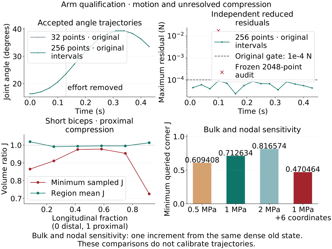
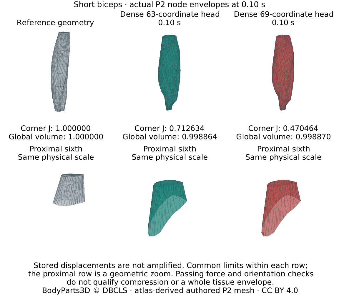
exact-domain scope
Change the stretch gradient and compensation; inspect the existing
closed prism mesh.
Algebraic local-volume claims do not prove mesh integration or
floating-point refinement.
Connect fibre architecture to force
without inventing strength
Worked example · 1 / 4
Calculate one reference-cut force
Use authored reference area 80 mm² and nominal stress 300 kPa. Their
product is 24 N along the fibres. At zero pennation all of that force
acts along the tendon direction.
Observe Reference and current-cut forces both read 24
N. This is analytic bookkeeping with prescribed stress, not measured
muscle strength.
Worked example · 2 / 4
Change area and stress together
Shorten to stretch 0.8 while imposing J=1. Current fibre-normal area
becomes 80/0.8 = 100 mm² and Cauchy stress becomes 300 × 0.8 = 240 kPa.
Observe 100 mm² × 240 kPa still gives 24 N. Shortening
alone does not change the prescribed nominal force in this example.
Worked example · 3 / 4
Project the force once
Keep the same material cut and turn the fibres to 30 degrees.
Tendon-directed force is the fibre force times cos(30 degrees).
Observe Axial and current-cut forces stay 24 N;
tendon-directed force becomes about 20.7846 N. Seven drawn lines encode
orientation, not a fibre count.
Worked example · 4 / 4
Check a familiar angle
At 60 degrees the projection factor is one half. Projecting both an
already projected area and the force again would apply the angle twice.
Observe Tendon-directed force is 12 N while axial force
remains 24 N. The orange cut slab is a diagram; the reported area is
analytic.
The unresolved anatomical requirement is a source-bound map from
fibre architecture and measured force to the active continuum
coefficient. Kenoma currently fits model-reference actuator forces while
its calibration states retain unresolved stationarity and compression.
That fit must not be renamed physiological specific tension.
After the prescribed local-volume map and before material response,
this lesson supplies the bookkeeping prerequisite: distinguish fibre
number from fibre area, parallel groups from sections in series, nominal
from Cauchy stress, and projected from unprojected PCSA. It does not
repair the continuum solve or supply a new anatomical dataset. All lab
numbers are authored examples, not calibration inputs.
Retain the failed
calibration evidence
At PR11
commit 0bed56a, the fixed-end fits use approximately 3.60, 8.71, and
20.38 MPa for brachialis, short biceps, and long biceps. The source
documents corner volume ratios near 0.56–0.62 and free nodal force
components of 64.07, 52.06, and 54.22 N at those frozen calibration
states. A successful reduced force match is therefore not an
equilibrated full-nodal material calibration.
This book integration adds six scoped Real claim registrations and a
portable analytic lab. No fit, material coefficient, calibration state,
accepted trajectory, reference asset, or failure threshold is changed.
Resolving local compression and full displacement/pressure stationarity
remains an upstream gate. The analytic examples below cannot overrule
it.
Decide which area a
measurement describes
For a declared parallel reference bundle with volume V₀ in m³,
representative fibre length Lf₀ in m, and contractile volume fraction
φ₀, the idealization Acontractile₀ = φ₀ V₀ / Lf₀ gives area in m². It
requires a meaningful representative length and fraction. A tapered
whole belly, distributed fibre terminations, varying orientations, or
nonuniform packing need a spatial integration and load-path model;
inserting their total volume into this formula does not establish those
conditions.
PCSA definitions must travel with the values. Murray,
Buchanan and Delp (2000), Methods and Table 2 computes PCSA from
volume divided by optimal fascicle length, then uses the pennation
cosine separately in moment capacity. Its elbow architecture study used
ten upper extremities from nine cadavers, with exclusions and different
sample counts by muscle. In contrast, Ward and
Lieber (2005), equation 1 includes the cosine in PCSA. A projection
included in an imported area must not be multiplied again.
Use three explicit metadata fields before combining a force and
area:
area convention: fibre-normal or already tendon-projected
stress basis: contractile area or an effective whole-muscle
area
configuration: reference/optimal or current, with the stated stretch
and volume ratio
An effective whole-muscle specific tension may already include
noncontractile fractions through its area definition. Multiplying it by
φ₀ again double-counts that reduction. Conversely, a single-fibre
measurement does not automatically define a whole-muscle effective
stress. A smallest fibre diameter is not a measured circular
cross-sectional area, and a fibre count fraction is not an area
fraction.
Sum parallel fibre groups by
area
For group k with Nk fibres, reference fibre area ak₀, nominal axial
stress Pk, and current tendon-direction cosine ck, use
A₀ = Σk Nk ak₀
T = Σk Pk Nk ak₀
Ttendon = Σk Pk Nk ak₀ ck
This is a declared independent parallel-force decomposition. It omits
passive matrix force, pressure traction, lateral exchange between
groups, and curved aponeurosis geometry. It cannot infer recruitment or
force–velocity properties from fibre typing alone.
Two synthetic groups with equal counts of 50,000 and areas of 1,000
and 2,000 µm² have area shares 1/3 and 2/3. At nominal stresses of 100
and 300 kPa, total area is 150 mm² and force is 35 N. The count-average
stress gives 30 N and is the wrong weighting for this example. Different
angles likewise require force-weighted projections, not an unqualified
average angle.
Mattiello-Sverzut
and Martins (2023) assessed isokinetic elbow performance in 32
volunteers; usable biceps morphology samples came from 26 participants
(9, 8, and 9 across the three age groups). Fibre subtypes and smaller
diameters describe that morphology subset, not all 32 participants. The
study supports keeping type and size distinct; it does not provide a
subject-matched spatial packing map for the atlas. Bottinelli
et al. (1996) reports type- and temperature-dependent single
skinned-fibre mechanics. Its 12 °C load-clamp protocol is not a
body-temperature whole-biceps calibration. Neither paper’s parameters
are imported here.
Track the same
material cut during shortening
Let F be a locally homogeneous orientation-preserving deformation
gradient, J = det F > 0, f₀ a reference unit fibre, λ = |F f₀| >
0, and f = F f₀ / λ. For a reference cut normal to f₀ with area A₀, the
current oriented area vector is a = J F⁻ᵀ f₀ A₀. Its projection normal
to the current fibre is
A⊥ = a · f = J A₀ / λ.
A⊥ is a projected material-cut area. In a shear-free straight bundle
it is the familiar orthogonal cross-sectional area. With shear, the
actual deformed cut may be oblique and have a different surface area.
The formula is not a global statement about an anatomical imaging plane
or a curved heterogeneous belly. Spatially varying F requires local
integration.
The existing active law in anatomical-material.mjs
differentiates a full-stretch potential. With p = aactivation σ₀ fL(λ),
its active first Piola tensor is p f ⊗ f₀, and its active Cauchy tensor
is (p λ/J) f ⊗ f. Thus
σfibre = p λ / J
Tactive = σfibre A⊥ = p A₀.
Both p and σfibre have units Pa, but they divide force by different
areas. The lab calls the scalar p “nominal stress P” and keeps it fixed
initially. With A₀ = 80 mm², p = 300 kPa, J = 1 and λ = 0.8, A⊥ grows to
100 mm² and σfibre falls to 240 kPa. Axial force stays 24 N. At 30°
pennation the projected component is about 20.78 N. There is no
fibre-count increase and no extra bulge multiplier.
Default material-cut case
Reference contractile area
80.00 mm²
Current projected area
100.00 mm²
Nominal stress P
300.00 kPa
Cauchy fibre stress σ
240.00 kPa
Axial force
24.00 N
Tendon-directed component
20.78 N
Authored default: geometric reference area 100 mm², contractile fraction
0.80, fibre stretch 0.80, volume ratio 1.00 and pennation 30°. The
force–length multiplier is held at 1. The tendon-directed component is
rounded to two decimals.
Open the interactive
architecture-force lab. Change stretch, volume ratio, packing
fraction and pennation separately, then enable the authored force–length
curve and reset. The table remains readable in print and without
JavaScript.
Try and predict. With force–length held at 1, lower
the stretch while holding J and the reference bundle fixed. Predict the
new projected area and Cauchy stress before checking the unchanged axial
force. Reset, change only pennation, then compare the axial force with
its tendon-directed component. Finally enable the authored force–length
curve: explain which assumption changed. Changing packing compares
different reference bundles, not acute fibre creation.
Holding Cauchy stress fixed instead would produce a different force
as area changes. That is a different constitutive prescription, not a
universal strength bonus. Enabling the existing authored fL curve in the
lab explicitly changes p and therefore force. In the anatomical model,
activation, length, passive stresses, pressure and attachments jointly
matter; this calculation is only its active material-cut identity.
Raiteri,
Cresswell and Lichtwark (2016) examined human tibialis anterior with
three-dimensional ultrasound and found spatial shape and architectural
changes during isometric contraction. It motivates regional rather than
uniform geometry. It is neither biceps anatomy nor proof of exact local
J = 1. The volume controls here are prescribed and have no biological
acceptance range.
Follow a
variable cross section through a series load path
Under a one-dimensional static section resultant convention, a cell
between cuts i and i+1 obeys
Ti+1 − Ti + Qi = 0,
where Qi is net axial force from lateral or external loading on that
cell. With no lateral load or inertia, axial force is the same at every
cut. A 100–200–100 mm² reference-area sequence carrying 30 N therefore
has nominal section stresses of 300–150–300 kPa. A thicker middle
section does not manufacture an additional end force.
If one assigns 300 kPa independently to each cut, the resulting
30–60–30 N sequence needs −30 N and +30 N lateral forces in the two
intervening cells. Such exchange could belong to a resolved ECM/matrix
path, but it must be represented and balanced. It cannot be inferred
from the taper alone. The scalar sequence is a necessary force-balance
example, not a compatible displacement field, three-dimensional
equilibrium, shear-stress solution, or material fit.
Internal paired forces cancel in the whole-body resultant. Their
power does not generally vanish: q v₁ + (−q) v₂ = q(v₁−v₂). An ECM
coupling can store or dissipate energy when adjacent points move
differently. A no-slip tie, compliant bond, frictional slip and damage
law are distinct constitutive choices; none is supplied by the
arithmetic identity.
Huijing and Baan
(2003) found differing proximal/distal tendon forces in maximally
active rat extensor muscles with connective tissues retained and
controlled relative length changes. This is evidence for additional
force paths, not a human-biceps coupling coefficient. Zhang and Gao
(2012) used a two-dimensional fibre/endomysium model to study shear
transfer and tapered fibre ends. Its model supports the need to declare
interface mechanics; it does not calibrate Kenoma’s matrix.
Density and
fluid mechanics remain separate inputs
Mass density maps volume to mass, not area directly to force. Ward
and Lieber’s fixation/hydration experiment reported
preparation-dependent human muscle density and warned of PCSA errors
from mismatched assumptions. Their fixed-tissue results are not live
biceps density measurements. A later mass-based estimate must retain
species, tissue preparation, hydration and the density uncertainty
rather than silently treating 1,060 kg/m³ as universal.
Sleboda
and Roberts (2020) applied a pressure cuff during isolated bullfrog
semimembranosus contractions. The effect on measured force changed with
muscle length, and physical ECM analogues helped interpret the result.
The experiment does not identify a human biceps pressure law or a unique
mechanism. It does show why fluid–matrix interactions cannot be
represented by “more blood equals more strength.”
Intracellular/interstitial fluid, blood inside vessels, solid-matrix
stress, incompressibility pressure and measured intramuscular pressure
are different quantities. The original cat fast/slow muscle
pressure and perfusion study varied perfusion conditions and
examined isometric endurance. Its experimental scope requires vascular
boundary conditions and timescale-dependent physiology; a bulk penalty
contains neither. No numerical perfusion, permeability, ECM bonding,
blood-volume or edema parameter is imported in this lesson. Exercise
pump and chronic growth are not acute material-area transformations.
For a future coupled fluid model, record the conserved constituents,
fluid pressure definitions, permeability and boundary conditions,
vascular compartments, compressibility assumptions, and the
drain/undrain time scale. Validation must distinguish local from global
volume, and conservation from accurate geometry. A shared external
skin/fat envelope must enclose the assembled tissues and obey its own
interface/contact conditions; seven separately expanding bellies do not
define it.
Verification and next acceptance
gate
The preserved contribution has twelve Node contracts for scalar units
and transformations, explicit PCSA/packing conventions, heterogeneous
sums, taper equilibrium and lateral force balance. Its
repository-contract tests compare the active-stress map with the
unchanged material operator, including shear and rigid rotation. Seven
SymPy identities separately check declared algebra, including cofactor
projection and exchange power. Symbolic simplification and unit tests
are not Lean kernel proofs.
The six original claim IDs and theorem names are registered in this
book candidate. ArchitectureForce.lean is copied
byte-for-byte from the independently qualified contribution. The cards
state explicit assumptions and retain the original exclusions; the fresh
book checker must compile every registered family before issuing book
proof receipts. The historical nonuniform-volume integration was 103 + 6
= 109 declarations. Adding these six architecture-force contracts gives
a 115-declaration source inventory across fourteen files: 30 integer and
85 Real declarations. Source registration alone does not establish a
freshly checked 115-declaration book, a rendered PDF or hosted
release.
The bounded standalone contribution checks in run
37743673184, at exact commit
143ac8863cd8a5be736e2c455cac9605c2e20a1f, compiled all six
contracts and passed real Chromium controls at 1280×1000 desktop and
393×852 mobile sizes, including the no-JavaScript fallback. The recorded
agent visual review passed all five JPEG quality-85 captures. That
evidence applies to the standalone source; it does not qualify this
integrated book. Its original automated
pending human inspection marker remains historical
evidence, unchanged.
The portable lab adds default values for print and no-JavaScript
reading while preserving the model and control code. Original contribution
sources, primary-source
ledger and book
assembly binding keep source, test and evidence scopes distinct.
Statements in the preserved standalone documents about pending
registration describe that earlier stage. Integrated desktop/mobile
controls, PDF readability, complete proof closure, owner release review
and any publication remain separate gates. The full book build also
launches numerical experiments; it is not a render-only check.
The next anatomical implementation gate is still an equilibrated,
locally admissible calibration specimen with an adequate
displacement/pressure space. Only after that gate should a source-bound
architecture dataset be mapped into σ₀ or a replacement law. Every
proposed parameter should carry the source, specimen/protocol,
area/stress convention, units, uncertainty, transformation and
destination equation. Independent attachment, tendon, cartilage, fat and
shared-skin validation remain necessary for the full anatomical arm
goal.
Interactive 3D · Fibres, cuts and projected force
Analytic bookkeeping · related checked claims have separate exact-domain
scope
Change pennation and material stretch; compare reference and current cut
forces.
Authored areas/stresses; one projection only; no contraction or
calibrated muscle prediction.
Let material stiffness and
boundaries choose the lateral shape
Worked example · 1 / 4
Compare unloaded boundary conditions
Start at unit height with shear modulus 1500 Pa and bulk modulus 50000
Pa. Neither free sides nor unilateral walls need a reaction in the
reference state.
Observe Both J values and lateral stretch are 1; plate
forces and wall reaction are zero.
Worked example · 2 / 4
Impose the same height reduction
Shorten height to 0.8. The free specimen solves zero lateral traction
and expands sideways; the confined specimen is prevented from widening.
Observe Free lateral stretch is about 1.11463 and J is
0.993914, compared with confined J=0.8. Plate forces are about 4.53637 N
and 42.0887 N, respectively.
Worked example · 3 / 4
Change bulk stiffness without changing height
Increase bulk modulus fivefold while keeping the same geometry, shear
modulus and boundary conditions. The free specimen can preserve more
volume by expanding; the walls prevent that route.
Observe Free J rises to about 0.998781 and plate force
to 4.56728 N. Confined J stays 0.8 while its force rises to 202.089 N;
stiffness does not override the prescribed walls.
Worked example · 4 / 4
Read the residual before trusting a shape
Return to bulk modulus 50000 Pa but stop bisection after eight
iterations. The specimen still has positive volume and looks plausible,
yet its free-side traction is not balanced.
Observe Free lateral residual is about 24.0254 Pa,
above the unchanged 0.00001 Pa criterion, so Free converged is false.
Increase the cap manually to 64 to recover the second step.
Question: when a block is shortened between plates,
must its volume stay exactly fixed? The preceding isochoric
lesson imposed that answer. Here a material law and lateral boundary
conditions choose the shape. Compare both conditions at one prescribed
height, then change one stiffness at a time.
This is an authored, homogeneous elastic specimen, not measured
muscle. The reference width, height and depth are
m,
m and
m;
m³. Ideal frictionless plates prescribe height stretch
.
The single unknown lateral stretch
acts equally in X and Z:
This diagonal homogeneous ansatz rules out bulging, shear
localization, buckling and spatially varying fields. Uniform stress
makes the lateral traction condition meaningful within this ansatz; this
is not a mesh solve or a proof of the unrestricted specimen’s preferred
deformation.
An elastic energy,
finite stiffness and units
Reuse the existing homogeneous tissue
energy, leaving the earlier labs’ equations and calibration
unchanged:
Here
and
are shear and bulk parameters of this declared energy,
each in Pa = J/m³. They characterize the reference response;
finite-deformation tangent stiffness need not equal these constants.
Controls permit
Pa and
Pa. These are bounded teaching choices, not fitted biological ranges.
The
endpoint deliberately removes resistance to pure volume change.
A finite bulk term penalizes
with finite energy; it does not impose
.
The shear term penalizes distortional shape change and vanishes under
positive isotropic scaling. Neither term supplies plasticity, damage,
viscosity, fluid transport, fibre architecture or activation.
The constitutive framework has an original-author reference: A. F.
Bower, Applied Mechanics of Solids, §3.5 describes
hyperelastic stress as an energy derivative and distinguishes nominal
stress from force per deformed area. The formula and boundary reduction
here are the book’s illustrative model. No experimental response curve
is reproduced or calibrated from that source.
Quantity
Units
Meaning
dimensionless
Height stretch, lateral stretch, volume
ratio
J
Stored elastic energy for the whole
reference block
Pa
Nominal stresses and inward wall reaction
per reference side area
N
Compressive force on one height plate
Pa
Plate force divided by its current
area
m
Clearance between specimen and each
lateral wall
Derive the reduced
equilibrium
The nominal stress components computed from this energy are
Both lateral directions vary with
,
hence
;
.
Finite-difference tests check these derivatives and the reduced plate
force. Free sides require zero lateral traction,
.
The numerical root bracket is
:
the left endpoint has zero shear contribution and nonpositive bulk
contribution; the right has
and nonnegative shear contribution. Analytic endpoints handle
and
.
This bracket supports the implemented root search; no Lean proof of
existence, uniqueness, convergence or global optimality is claimed.
Unilateral confinement places smooth rigid walls at
the reference X/Z faces. Walls prevent outward expansion but allow
inward pull-away:
.
They apply inward compressive reaction
and cannot pull the block outward. The reduced wall contract is
At
,
if
,
use
and
.
Otherwise solve the free-traction root on the restricted bracket
and use
.
The separate bracket keeps even a finite approximation inside the walls.
At weak bulk stiffness, the specimen can shrink away from the walls;
forcing
in that case would require an unmodeled tensile attachment.
Plate force and pressure follow from the same nominal stress, not
from displayed arrows:
The sign convention makes compression positive. Each X wall carries
;
each Z wall carries
.
Their current-area pressure is
.
Per-wall clearances are
and
.
The reported complementarity work is
in joules, accounting for both walls in each direction.
Property lab 4 · Compression, bulk stiffness and confinement
Homogeneous quasistatic elastic equilibrium; shared prescribed height;
free sides versus unilateral rigid walls. Authored parameters, SI units;
no muscle calibration.
Solved homogeneous 80 × 60 × 50 mm reference block at height stretch
0.8, shear parameter 1,500 Pa and bulk parameter 50,000 Pa. Free: J =
0.993914, plate force 4.53637 N. Rigid unilateral walls: J = 0.8, plate
force 42.0887 N. Dashed outlines are reference; gold lines are
frictionless plates. Front view at one fixed physical scale; depth also
scales by lateral stretch b.
Front view of the solved blocks at the same height and fixed physical
scale. Dashed: reference. Gold: frictionless plates. Red walls:
compressive contact; gray walls allow pull-away. Both unshown depths
also scale by b. Numerical values are unscaled SI. Finite residual
success does not establish physical validity.
Predict,
change one input, and inspect the residual
At default
,
Pa and
Pa, the plate spacing is 0.048 m in both panels. These values come from
a fresh reduced solve:
Boundary condition
Lateral stretch
Volume ratio
Plate force (N)
Stored energy (J)
Free lateral surfaces
1.11462688
0.99391447
4.53637103
0.02497727
Unilateral rigid walls
1
0.8
42.08871498
0.25142075
Try and predict. Raise only
to 250000 Pa. The free block approaches
without imposing it:
,
while its plate force is about 4.56728 N. Active rigid walls retain
and
,
so the plate force rises to about 202.08871 N. Confinement changes the
work required to reach the same height; increasing finite bulk stiffness
cannot restore volume while all three stretches are fixed.
Restore
Pa and raise only
to 5000 Pa. Read the force, lateral expansion, and separate bulk/shear
energy contributions. Height remains shared. Every comparison changes
only the named input; no time or activation state is hidden in this
static lesson.
Counterexample. Set
.
The solved block has
,
and zero stored energy/plate force up to roundoff: at
,
.
Isotropic collapse costs no distortional energy in this deliberately
degenerate law. It is not a plausible soft-muscle response or plastic
failure. At
Pa, both solutions shrink laterally to
,
with zero wall reaction and positive clearance. Confinement does not
manufacture tensile attachment.
Feasibility check. The “Test isochoric wall
candidate” button tries
in the confined geometry. For
it has positive
but penetrates the lateral walls and is rejected without changing the
solved state. Positive volume is necessary but does not establish
boundary feasibility.
Numerical check. Select eight bisections. Geometry
remains positive and wall-feasible, but the signed free residual
generally fails the displayed criterion
Pa. Restore 32 or 64 and compare the bracket width and residual. The
criterion belongs to this new lesson; it changes none of the existing
labs’ acceptance limits. “Residual criterion met” refers only to this
reduced lateral equation. Invalid, blank, nonfinite or out-of-domain
inputs retain the prior displayed state.
Finally restore
:
,
,
energy and force return to zero. This model has no history or
irreversible state, so it cannot demonstrate plastic deformation or
dissipative load/hold/release. Reset deliberately restores all authored
defaults.
Real
properties: checked algebra and unfinished formal obligations
The specimen uses real stretches, stresses and
energies. Five real-domain algebra claims below are compiled against the
pinned mathlib dependencies before this book is built. Constitutive
derivatives and equilibrium existence, uniqueness and optimality remain
unfinished. The separate integer contracts do not
substitute for these real claims or their remaining obligations.
Real claim and assumptions
Derivation in this lesson
Real formal status
,
imply
Substitute into
Checked real substitution
,
imply
;
for
it vanishes exactly at
A real square is nonnegative; a product
with positive factors vanishes only when the square does
Checked real bulk algebra
and
imply
Divide the assumed complementarity
equation by nonzero real
Checked real implication; complementarity
is assumed, not certified
,
for positive stretches
Differentiate the stated energy with
and
Unfinished; real powers and derivatives
need formal support
Lateral virtual work factors as
Add the two equal lateral stress and wall
contributions
Checked real factorization; does not
establish equilibrium
The earlier real determinant and square-root identities support the
kinematic volume formula. They do not prove this constitutive law, wall
solution, equilibrium existence/uniqueness or global optimality. A
release build must compile any future real-domain claim with its
supported pinned dependencies before presenting it as checked.
Discrete
arithmetic contracts and separate numerical evidence
The five declarations below are freshly compiled with pinned Lean
4.19.0 and bundled Std. They concern exact scaled
integers, with positive external SI scaling factors. These are
separate implementation arithmetic checks; real stretches, stresses and
energies are not their quantified domain. The unfinished derivative and
equilibrium obligations above remain separate.
Numerical tests independently derive a stationarity equation in
,
check energy derivatives and SI conversions, sweep the bounded controls,
compare feasible energy samples, and exercise finite caps, wall onset,
zero bulk and invalid candidates. Browser tests execute the generated
controls, verify exported states and SVG dimensions at a common physical
scale, and check rollback, reset, mobile/print and no-JavaScript
alternatives. These tests establish behavior for this declared
implementation, not global optimality, mesh accuracy, material
calibration or biology.
Continue with anatomical evidence
before attaching these parameters to a named muscle. Laboratory 5 later reuses the
free-side law in a coupled hinge example. The unfinished anatomical
capstone, measured fibre-to-muscle aggregation, force–length/velocity
lessons retain their separate limits in the coverage chapter.
Interactive 3D · Free and confined compression
Numerical demonstration · related checked claims have separate
exact-domain scope
Change height stretch and inspect free versus confined lateral response.
Existing homogeneous one-lateral-DOF equilibrium; not unrestricted 3D
material stability.
A one-second ramp raises the axial force to 0.6 N. Work splits into
recoverable storage and viscous loss; both quantities come from the
existing standard-linear-solid protocol.
Observe Extension is about 1.68159 mm. Work 0.000531635
J equals storage 0.000434748 J plus loss 0.0000968864 J up to roundoff.
Worked example · 2 / 4
Hold force and observe creep
Keep force at 0.6 N during the hold. Extension keeps increasing, so the
load continues doing work as the viscous branch evolves.
Observe Extension grows to about 2.32895 mm while force
remains 0.6 N. Storage plus accumulated loss still matches the displayed
external work.
Worked example · 3 / 4
Change what the fixture holds
Replay from the same initial state and loading ramp, but hold extension
after 1 s. With no further extension during the hold, no additional
external work is done.
Observe Extension stays 1.68159 mm; force relaxes to
about 0.402942 N. Work remains 0.000531635 J while storage decreases and
loss increases.
Worked example · 4 / 4
Release and inspect finite recovery
Return to the force-hold protocol and inspect its end after unloading
from 3–4 s and recovery from 4–7 s. Zero applied force does not imply
instantaneous recovery.
Observe Force is zero, but residual extension is about
0.189097 mm and storage about 0.00000773842 J. Loss is 0.000511623 J;
the finite run does not claim complete recovery.
The axial
bar lesson made area and elastic strain visible. Keep its passive
force balance, area profiles and equilibrium modulus, then add one
internal strain that takes time to change. The learning objective is to
distinguish creep under held force from stress
relaxation under held extension, and account for recoverable
storage, signed external work and viscous loss throughout unloading.
The bulk/shear
compression lesson remains a separate finite-deformation model. This
lesson follows the earlier small-strain axial bar: fixed material
reference area
,
homogeneous axial coefficients, no body force, inertia, transverse
equilibrium or active stress. Displacement and strain have
tensile-positive signs. It uses a standard linear solid: an equilibrium
spring in parallel with one Maxwell spring–dashpot branch. Roylance’s MIT
teaching notes, §4.2 present this arrangement and distinguish creep
from relaxation. COMSOL’s
constitutive theory describes the same one-branch topology and
viscosity/time-scale relation. These sources motivate the model; the
coefficients below are authored demonstrations, not measurements of
human tissue.
One law for the image and
the ledger
Let
be total axial strain and
the viscous strain in the dashpot. The Maxwell spring strain is
.
With fixed
,
and
,
Here
have units Pa and
has units Pa s. This adds memory to the passive axial law. Setting
recovers
and the earlier bar’s same midpoint strain, displacement and stored
energy for identical geometry and load.
The stored energy density and viscous loss rate density are
Differentiation and the Maxwell equation give the local balance
For the whole bar,
,
and external power is
.
Work
is signed; unloading can return energy to the apparatus.
is cumulative lost mechanical energy and cannot decrease. Starting from
rest gives
,
with the observed finite-precision residual displayed separately.
Constant force
balance and an internal state
With constant resultant
,
.
Uniform coefficients and an initially unstrained bar imply
and
,
where
have units m². Define the geometric compliance factor
,
with units 1/m. Then
Under imposed force,
Holding force therefore permits increasing extension. Holding
extension fixes
;
then
and force relaxes. For elapsed hold time
,
The relaxation time is
and the force-controlled creep time is
when
.
With the default equal moduli, these are 1 s and 2 s. Increasing
viscosity delays response; it does not imply a monotone change in energy
lost during every finite protocol.
The runtime integrates the scalar state exactly for each
constant-extension interval and each linear force ramp. It separately
integrates boundary work and squared viscous rate; loss is
not filled in from the energy residual. Stable
exponential differences avoid cancellation near
.
Each step clips at protocol boundaries before changing the imposed
condition. The bar uses explicit midpoint area quadrature. For a linear
taper, the independent factor is
with limit
at
;
for two equal-length segments,
.
The displayed refinement error compares midpoint extension to this exact
profile integral.
Run the same finite protocol
Default reference:
m,
m², area ratio
,
Pa,
Pa s and 32 midpoint cells. Load ramps from 0 to 0.6 N over 1 s, holds
for 2 s, unloads from the actual reaction to zero over 1 s, then
recovers at zero force for 3 s. Switching to extension hold captures the
extension reached at the end of loading. The unloading ramp begins at
the relaxed reaction. Both switches preserve extension and internal
state continuously.
Default force-controlled load, hold,
unload and recovery. Axial displacement is magnified tenfold; reference
scale stays fixed.
Property lab 5 · Creep, relaxation and viscous loss
Small-strain quasistatic axial standard linear solid: equilibrium spring
in parallel with a Maxwell branch. Ramp, hold, unload and zero-force
recovery expose history dependence. A force hold gives creep; a held
extension gives force relaxation. Authored coefficients; no transverse
equilibrium or muscle calibration.
Reference length 0.2 m; area A1 = 0.0003 m²; equilibrium modulus E0 =
100,000 Pa. E1 = 0 recovers the passive elastic bar.
Each parameter edit starts a new experiment: time,
internal strain, work, loss and trace reset; playback pauses. Invalid
entries retain the prior experiment.
Axial displacement is enlarged exactly ×10 at a fixed reference scale.
Cell height shows reference area divided by a 0.01 m diagram depth;
transverse deformation is not solved. Strain colors use one fixed
palette: −0.05 +0.05. SI readouts are unscaled.
Hold
Time (s)
Force (N)
Extension (mm)
Stored U (mJ)
Signed W (mJ)
Loss D (mJ)
creep
0.0
0.000000
0.000000
0.000000
0.000000
0.000000
creep
1.0
0.600000
1.681586
0.434748
0.531635
0.096886
creep
3.0
0.600000
2.371154
0.625806
0.945376
0.319569
creep
4.0
0.000000
0.847472
0.155430
0.519361
0.363931
creep
7.0
0.000000
0.189097
0.007738
0.519361
0.511623
relaxation
0.0
0.000000
0.000000
0.000000
0.000000
0.000000
relaxation
1.0
0.600000
1.681586
0.434748
0.531635
0.096886
relaxation
3.0
0.395869
1.681586
0.308339
0.531635
0.223296
relaxation
4.0
0.000000
0.630197
0.085948
0.336306
0.250357
relaxation
7.0
0.000000
0.140616
0.004279
0.336306
0.332027
During force hold, compare the extension at 1 and 3 s. During
extension hold, compare those forces instead. During the latter hold,
boundary work stays constant while spring storage decreases and
rises. At 4 s the applied force is zero, yet extension and stored energy
remain positive. Recovery consumes that storage through viscous loss. At
finite time 7 s a residual extension remains; the figure does not
declare full recovery.
Try viscosity 20,000 and 500,000 Pa s, then change the ramp duration
while retaining the same force target. Compare the same protocol
boundary times and read
,
,
and the residual separately. Set the Maxwell branch off: there is no
viscous loss, force hold no longer creeps, and restoring zero force
restores zero strain and storage. Reverse the taper or use two
equal-length areas; the strain field and extension change through
while the same constitutive law remains in force.
The scene uses a fixed physical reference scale, explicitly magnifies
axial displacement tenfold, and colors strain against a fixed ±5% scale.
Thickness is schematic; there is no predicted lateral contraction.
Changing a model or protocol parameter deliberately starts a new
experiment and clears time, memory and energy history. Invalid edits
retain the prior valid state. Reset restores the authored defaults. Step
and Play advance physical time; Run completes the bounded protocol in
small animation-frame batches. Export includes the initial row and every
accepted observation.
Controls restrict positive geometry, equilibrium modulus at least
100,000 Pa, force at most 0.6 N and area ratio at least 0.5. The true
narrow-end strain remains at most 4% in these tensile protocols, below
the unchanged 5% small-strain warning used in the earlier axial lesson.
The runtime rejects inconsistent constitutive state, imposed-force
schedules, held extension or energy ledger rather than transferring an
arbitrary state to new coefficients.
What the real proofs
establish
The eleven declarations below quantify real local constitutive
variables. They check storage and loss signs, the storage derivative
given path derivatives, power balance assuming the
Maxwell equation, the zero-branch elastic limit, and the exact
held-strain exponential’s derivative, bounds and weak monotonicity. They
do not prove the force-controlled bar reduction, midpoint quadrature,
JavaScript arithmetic or exported discrete energy ledger. Independent
numerical and actual-control checks cover those implementation
obligations separately. No anatomical calibration, force–velocity muscle
law or completed capstone follows from this example.
Continue to anatomical evidence
before deciding which properties a named tissue would need. The
anatomical capstone and its calibration obligations remain separate.
Continue with unequal blocks under
one force to connect finite force-driven stretches, current areas
and local incompressibility in a separate two-block 3D assembly. The SLS
law and energy history above remain unchanged.
Interactive 3D · Load, hold and recovery specimen
Numerical demonstration · related checked claims have separate
exact-domain scope
Scrub the existing finite SLS protocol and compare work, storage and
loss.
One-dimensional small-strain bar extruded for viewing; transverse area
is not solved.
The second reference cross-section is twice the first. A massless spacer
transmits the same axial force and allows the blocks to slide laterally
at their ideal fixtures.
Observe Both stretches and measured volume ratios are
1; current areas are 300 and 600 mm². The gap and grey connector
represent the spacer, not missing tissue.
Worked example · 2 / 4
Transmit one tensile force
Apply +0.1 N to both blocks. The narrower block needs twice the nominal
stress, so the same neo-Hookean law gives it the greater stretch.
Observe Stretches are about 1.07983 and 1.03844;
current areas shrink to 277.821 and 577.788 mm². Each measured volume
ratio remains 1.
Worked example · 3 / 4
Reverse the signed load
Apply −0.1 N using the same bilateral fixtures. The narrower block now
shortens more and expands more laterally; neither block changes its
local volume.
Observe Stretches become about 0.931143 and 0.964301;
areas become 322.185 and 622.212 mm². The shared force does not imply
equal stress or equal strain.
Worked example · 4 / 4
Expose finite root error
Restore tension but reduce the bisection cap to eight. Incompressibility
remains imposed exactly while axial force balance is only approximated.
Observe The maximum force residual is about 0.00164715
N, above the 1e-10 N criterion, so Converged is false even though both
volumes are preserved.
Question: can blocks of the same material carry the
same force, stretch by different amounts, and each preserve volume? The
reduced
axial bar already demonstrates uneven strain from an input area
profile, including local extension and compression under fixed ends. It
predicts no lateral deformation. This lesson adds a different,
explicitly three-dimensional specimen and a constitutive law whose
force, current area and local volume agree.
Two blocks and an explicit
interface
Use two separate, homogeneous rectangular blocks in axial series.
Each has a square reference section and reference length
m. Their reference areas are
m² and
,
with default
.
Ideal bilateral axial traction fixtures transmit signed
force and permit tangential sliding at the loading faces. They can pull
or push; ordinary frictionless compression platens alone could not
provide the tensile case. A massless spacer has fixed length 0.012 m.
Its positions move with the block ends.
The two blocks may therefore change lateral size independently. The
gold fixture connection is excluded from material volume. This is an
assembly of separate blocks, not a continuous stepped or tapered solid
with an unmodeled material interface. The solved deformation is
homogeneous within each block. Buckling, shear localization and the
preferred deformation among unrestricted 3D fields are outside this
homogeneous model.
With no body load, the intervening massless fixture balances the two
opposing axial resultants, so
.
Positive
is tension and negative
is compression. The equilibrium equation uses reference
area for nominal stress, and current area for Cauchy stress; these are
different stress measures.
Material response
and the volume constraint
Each block is an incompressible isotropic neo-Hookean solid with
authored shear parameter
Pa. Its energy per reference volume is
Incompressibility is a local material constraint. It
is not a finite bulk penalty, and constant force does not establish it.
The earlier bulk/shear
confinement lesson retains its different finite-bulk law and
boundary conditions. The material framework and the role of
incompressibility pressure are described by A. F.
Bower, Applied Mechanics of Solids, §§3.5.4–3.5.6. The
following homogeneous reduction and assembly are the model used
here.
For axial stretch
and equal transverse stretches
,
The full Cauchy stress is
,
where
.
Free lateral faces require
,
giving
.
This
is an incompressibility multiplier, not measured axial
plate pressure. At rest it is
,
while the complete stress tensor is zero. The resulting axial Cauchy and
nominal stresses are
The executable root solves this last equation separately for both
blocks. It does not assign stretches from a visual taper. The reduced
energy and its derivative use the same material law:
Thus
,
and differentiating with respect to current block length
gives
.
The response is elastic and history-free; no time integration,
activation or viscous loss is added.
Solve, measure, and compare
For positive stretch and
,
The force curve is strictly increasing, with zero force at
.
The narrower section has larger nominal tensile stress and larger
stretch for
.
With
it has more negative stress and smaller stretch: it compresses more.
Both blocks have the same material; this difference comes from
geometry.
The current geometry is calculated from the solved stretches:
The 3D meshes use these actual lengths, widths and depths without
displacement magnification. Gray wire outlines mark the reference
blocks; the camera uses a shared physical scale across parameter edits.
Front/oblique views change the camera, not the model. Exported vertices
drive a separate closed-triangle volume measurement. Measured
cross-sectional edges, length and boundary volume are reported beside
;
the volume oracle does not simply return one.
Solved default tension, rest and
compression at one physical scale. Dashed outlines are reference blocks;
the moving gold spacer is excluded from material volume.
Property lab 6 · Force, current area and local volume
Two separate homogeneous square prisms in axial series, with ideal
bilateral traction-distributing fixtures that allow lateral sliding. A
fixed-length massless spacer moves with their ends. This is an assembly
of two blocks, not a continuous stepped solid.
Default reference length L0 = 0.025 m for each block; the length control
changes both reference lengths. Exact incompressibility is a
constitutive assumption: b = 1/√λ and J = λb² = 1. The pressure
multiplier p = μ/λ makes the lateral Cauchy stresses zero. Closed-mesh
volumes are measured separately; their constancy does not choose the
axial equilibrium.
Static parameter edits reevaluate the displayed signed force. Reference
geometry edits define a new specimen, so its reference volume can
change. Invalid inputs retain the last valid state. A low root cap shows
its actual force mismatch; it does not qualify equilibrium.
Static undeformed reference. Current numerical results appear below;
this diagram does not move.
Live mesh coordinates are metres with no displacement magnification.
Fixed physical camera; grid spacing 0.01 m. Gray wireframes show
reference blocks; dark outlines are ideal sliding fixtures; gold line is
the fixed 0.012 m spacer. Only block volumes are counted. Force arrows
show equal and opposite target applied N, at a fixed
0.1 N → 0.02 m symbol scale; low-cap cell resultants are reported
separately. Colours use a fixed strain scale: compression −0.4, neutral
0, extension +0.75.
Drag the live canvas to orbit; right-drag to pan. Front and Oblique
restore fixed comparison views. Two homogeneous constrained scalar
roots, not a 3D mesh solver, continuous interface solution, unrestricted
stability result or anatomical calibration.
Default forces, areas, stretches and independent measured volumes are
generated from the same executable law:
Load (N)
Block
Stretch λ
Axial strain
Area (mm²)
Volume (mm³)
Force residual (N)
0.100
1
1.079830
0.079830
277.821
7500.000
2.22e-15
0.100
2
1.038443
0.038443
577.788
15000.000
1.6e-15
0.000
1
1.000000
0.000000
300.000
7500.000
0
0.000
2
1.000000
0.000000
600.000
15000.000
0
-0.100
1
0.931143
-0.068857
322.185
7500.000
-2.39e-15
-0.100
2
0.964301
-0.035699
622.212
15000.000
5.58e-15
Try and predict. Reverse
from +0.1 to -0.1 N. Both blocks shorten and widen, and the narrower
block has the larger compression. Set
:
both stretches, areas and lengths return to their reference values, and
stress and energy vanish. Set
:
equal material and area give equal stretches. Reverse the ratio to
:
block 2 becomes the narrow section and now strains more. Increase only
:
at the same force the stretches move closer to one. Reference length
changes total extension, volume and energy, but does not change local
stress or stretch at fixed area and force.
Local-volume counterexample. The test button
constructs an unused candidate with unchanged axial stretches but local
volume ratios 1.10 and
.
Their reference-volume-weighted total is still one. Nevertheless, each
block violates
,
and its free-side traction no longer vanishes. The candidate is rejected
and the prior solved mesh and state remain visible. A correct total
volume cannot hide a violation of this local material law.
Controls bound
Pa,
m²,
,
N, and
m. Every target force lies within the fixed positive bracket
:
at the smallest
N its endpoint forces are approximately -0.163333 and +0.106760 N.
Bisection uses a visible 8–64 iteration cap. The force criterion is
N for each block. Eight iterations can leave a valid
positive-volume shape with unequal approximate resultants; the UI
reports each computed resultant and residual, rather than calling it
shared-force equilibrium. Restore 48 or 64 and compare. Invalid edits
retain the prior valid specimen; Reset restores the authored defaults
and reference camera.
Exact
real claims and independent implementation checks
Twelve declarations below quantify the actual real homogeneous law.
They prove the energy factor, sign and zero state; its derivative;
stress identities and signs; strict monotonicity and conditional
positive-root uniqueness; area-times- length volume; and same-force
ordering for unequal areas in tension and compression. Root existence,
numerical bisection, pressure elimination, the matrix/mesh volume
measurement and JavaScript arithmetic are not certified by these
declarations. The real kinematic identities in the first property
lessons remain separate.
Independent numerical checks solve the cubic equation
,
sum tetrahedral volumes from the actual mesh, differentiate the stored
energy, and verify the complete stress and current-area conversions.
Actual browser controls must also verify the displayed 3D geometry,
solver status, local-volume rejection and fallbacks. These obligations
cannot be replaced by a scope label. The lesson makes no claim about
measured muscle, continuous fibre aggregation or the unfinished
anatomical capstone.
Interactive 3D · Two separate blocks in series
Numerical demonstration · related checked claims have separate
exact-domain scope
Change transmitted force and compare the two solved stretches and areas.
Two separate homogeneous incompressible blocks and ideal spacer; not a
continuous tapered body.
Select the right humerus before assigning any material property. Its
2,233 vertices and 3,784 triangles identify the selected source
representation, not a stiffness, cartilage field or joint axis. The
display rotates the atlas frame only.
Observe Only the humerus is visible. Its name, original
OBJ hash and topology counts remain available beside the scene.
Worked example · 2 / 3
Separate a muscle surface from its architecture
Now isolate the short head of biceps brachii. The 1,739 source vertices
bound an atlas surface; they do not reveal fascicle direction, tendon
slack length or maximum force. Those would require separate measurements
or declared model assumptions.
Observe The selected surface and provenance change to
the short biceps head: 1,739 vertices and 1,856 triangles. No fibre or
force field appears.
Worked example · 3 / 3
Assemble evidence without inventing a subject
Restore the three bones and seven muscle surfaces in their shared atlas
coordinates. This is a constructed reference atlas, independent of the
recorded OpenArm participant and the Arm26 actuator model. Coincident
display is not registration.
Observe The ten surfaces retain 13,852 vertices and
20,218 triangles. Subject registration and clinical validation both read
false.
The previous laboratories isolate mechanics. An arm introduces three
descriptions that must agree: rigid skeletal geometry, force-producing
musculotendon paths, and deformable tissue. The humerus, radius and ulna
are distinct bones. Elbow bending and forearm rotation are distinct
motions; the biceps’ distal attachment to the radius makes this
separation important. Our next laboratory fixes forearm rotation and
shoulder posture and replaces the elbow complex with one hinge. Its rods
are teaching geometry, not segmented bones.
Name the
structures before assigning properties
The anterior volume includes biceps and the deeper brachialis;
brachioradialis contributes a separate lateral path. The triceps heads
provide extensor paths, and some muscles span the shoulder as well as
the elbow. A single red actuator cannot identify their individual
contributions. The chapter’s synthetic flexor is deliberately called a
synthetic flexor, rather than assigning its invented
origin and insertion to a named anatomical muscle.
An attachment region, a segmented surface, a tendon guide point, and
a fiber direction field are different data. The surface of a muscle does
not tell us how its fascicles run or where a numerical routing point
should be placed. An anatomical fascial expansion such as the bicipital
aponeurosis also needs an attachment/interface model; drawing another
cable is insufficient. The audited anatomy contribution supplies
anatomical literature and distinctions, but no imported mesh in this
edition establishes those features for our schematic.
Published human
numbers with their context
Murray, Buchanan and Delp examined ten human upper-extremity
specimens. Measurements included architecture and tendon excursion;
optimal fascicle lengths and physiological cross-sectional areas (PCSA)
were then estimated. Their Table 2 gives the following study summaries.
These are published biological estimates, not this laboratory’s
defaults, and no participant-level raw data are redistributed.
Original study, Table 2 and §3
Reported quantity
Study summary
Interpretation
Brachioradialis optimal fascicle
length
17.7 cm; SD 3.0 cm
Architecture estimate in the study
specimens
Brachioradialis PCSA
1.2 cm²; SD 0.6 cm²
Estimated parallel contractile area
Combined triceps PCSA
14.9 cm²; SD 6.7 cm²
Aggregate reported for combined heads
Convert 17.7 cm to 0.177 m and 1.2 cm² to 0.00012 m² before
calculations. For a uniform architecture idealization, PCSA is volume
divided by optimal fiber length. If maximum tendon-directed force is
modeled as specific fiber tension times PCSA times cos(pennation), check
whether the source already includes that cosine in its area convention.
The segmented volume and PCSA do not themselves specify a maximum force:
a specific-tension assumption is still needed.
Iivarinen and colleagues measured forearm indentation in nine healthy
people, used ultrasound for tissue thickness, and fitted a layered
hyperelastic model. Their resting effective moduli were 210 kPa
for skin and 1.9 kPa for adipose tissue,
equivalent to 210,000 Pa and 1,900 Pa. These are inverse-model values
under that study’s loading and layer assumptions. They are not universal
tissue constants or an elbow-contact calibration. Neither value is
inserted into the schematic hinge. Original abstract and DOI
The distinction matters: a measured displacement, a parameter fitted
from that displacement, and a new model’s prediction are three separate
objects. Testing the fitted model on its fitting observations is
calibration. Testing on a reserved pose or load is a stronger check of
generalization.
A dataset must say what it
observes
The audited research identifies several useful routes to actual data.
The table records research-stage access, not completed integration into
this executable.
Resource
Observations or content
Boundary and licence evidence
Visible Human
Cadaver cryosections, CT and MRI
Source images differ from derived
segmentations; official public-domain access description
BodyParts3D
Reference anatomical geometry and
anatomical identifiers
Official current archive CC BY 4.0;
preserve exact acquired version and attribution
OpenArm 2.0
Ultrasound-reconstructed biceps/arm
volumes over poses and loads
Research audit: eleven participants, CC BY
4.0; registration and predicted-label quality need review
OpenArm Multisensor 2.0
Ultrasound, EMG, force and task
information
Research audit: CC BY 4.0; modalities
concern different muscles; apply release errata
Quesada upper-limb dataset
EMG, kinematics and joint-torque time
series
Research audit: CC BY-SA 4.0; torque is
not measured individual muscle force
Arm26
Educational OpenSim model with six
actuators
Embedded model CC BY 3.0; educational
geometry/actuators differ from this one-hinge model
The following data chapter integrates a specific licensed Multisensor
trial after a reviewed passive conversion, preserving normalized values
and actual relative timestamps. Ordinary untrusted pickle
deserialization is unsuitable; no pickle is bundled or executed here.
The acquired atlas, recording and model parameters remain visibly
separate from the published study summaries above and from the schematic
actuator.
The current MoBL-ARMS package has a noncommercial restriction
according to the audited provider page, conflicting with an older
catalogue’s MIT label. It is excluded. Apache-2.0 on Kenoma code does
not relicense any dataset, model, mesh, scan, or paper figure. Data access and licence sources
Expertise follows the
contribution
Murray, Buchanan and Delp’s original architecture experiments are
relevant to architecture and moment capacity. Millard, Uchida, Seth and
Delp’s actuator comparisons are relevant to musculotendon modeling.
Wakeling, Ryan and colleagues’ continuum work is relevant to
force/deformation coupling. Hallock’s OpenArm research is relevant to
imaging-derived muscle deformation. These are source-based areas of
contribution, not endorsements of Kenoma or claims that any author
reviewed it.
No audited source supplies a complete, co-registered loaded curl with
all bones, fibers, activation histories, skin self-contact and pressure.
The book therefore keeps the evidence gap visible while building
mechanisms that can later be compared with compatible measurements.
Interactive 3D · Anatomy as source geometry
Recorded evidence · related checked claims have separate exact-domain
scope
Select a licensed atlas structure and inspect its original surface and
identity.
Static atlas; no posed anatomical rig or subject-matched muscle
parameters.
The recorded trial’s ultrasound channel observes brachioradialis
thickness. Isolate the atlas brachioradialis to learn the anatomical
name, while keeping the datasets separate: this surface is not a scan of
participant 2.
Observe The selected reference is brachioradialis with
3,270 vertices and 4,874 triangles. Subject registration remains false;
the atlas does not deform to the trace.
Worked example · 2 / 3
A second signal can concern a different muscle
The trial’s sEMG channel concerns biceps brachii. This selected
long-head atlas surface is an anatomical illustration, not localization
of the electrode or an isolation of that head’s signal. The recorded
values are normalized unit-one quantities, not activation or
individual-muscle force.
Observe The display changes to the long biceps head.
There is no conversion from the normalized recording into this surface’s
force or deformation.
Worked example · 3 / 3
Read three evidence streams without joining them
The chapter’s recorded curves, six Arm26 actuator parameter sets and ten
atlas surfaces answer different questions. The recording uses 4,403
irregularly timed samples and 172 half-second display bins; its held 90°
posture is not a measured angle trajectory. Read the existing plots and
source tables below alongside the unregistered atlas.
Observe All atlas parts return. No synchronization,
participant-specific fit or Newton-valued force is inferred from the
normalized recording.
An atlas, a recorded human trial and an actuator model answer
different questions. This chapter includes actual licensed data
bytes, with their source-specific rights, transformations and
hashes. None of the three evidence streams is registered to either of
the others or to the teaching actuator. Looking more anatomical cannot
turn a schematic force law into a validated physiological model.
Ten static anatomical
surfaces
Two anterior-facing views of a straight
right-arm atlas: humerus, radius and ulna alone, then seven selected
muscle surfaces with keyed colors.
Ten BodyParts3D 4.0 right-arm surfaces preserve the original atlas
pose: humerus, radius, ulna, brachialis, brachioradialis, both biceps
heads and three triceps heads. The official 99%-polygon-reduced release
supplies 13,852 vertices and 20,218 triangles. It is a constructed
static adult-male reference atlas, rather than scanned geometry for the
OpenArm participant. Rendering colors are explanatory. Source axes are x
toward anatomical left, y posterior and z superior; original OBJ
positions are in millimetres. The JSON divides positions by 1,000 and
converts face indices to zero-based, with no topology editing, joint
fitting or rigging.
The browser viewer centers and rotates the atlas for display
only. It can show bones or individual named parts, and switch
anterior, oblique and posterior views. It does not animate a guessed
elbow axis. Polygon reduction and edge diagnostics do not establish a
mesh suitable for medical contact calculations. No skin, fat, fascia,
cartilage or tendon material field is provided.
One recorded trial at a
held posture
Three aligned recorded curves over about
86 seconds: normalized brachioradialis thickness, biceps sEMG and
wrist-contact force, with different amplitudes and
profiles.
OpenArm Multisensor 2.0 participant code 2, trial 1b, was recorded
with the right elbow held at 90° and the forearm supinated. The retained
segment contains 4,403 preprocessed normalized samples over 85.903537 s.
Ultrasound measures brachioradialis thickness; sEMG
measures biceps brachii electrical activity;
wrist-contact force is a net external signal. They are different
quantities and, for ultrasound and sEMG, different muscles. The fixed
acquisition posture is not a measured angle trajectory. Hallock et
al. (2021), DOI 10.1109/TNSRE.2021.3133813; data CC BY 4.0. Changes:
selected trial/segment, relative timestamps, display binning and
original plot.
The source’s retained Processed values are already
trial-calibrated. Zero refers to relaxed calibration and one to its
calibration contraction: (signal − relaxed mean)/(MVC mean − relaxed
mean). The package does not normalize them again or clamp values outside
[0,1]. Their amplitude unit is one, not metres, volts
or newtons. Calibration to those physical units is not established, and
sEMG is not labeled activation a or individual-muscle force.
The saved timestamps are irregular. The segment averages 51.243524
saved samples/s despite the protocol’s nominal best-effort 1 kHz
description. The display uses 172 half-second bins, each [start,end),
with sample-weighted arithmetic means and the actual mean sample time;
the last bin can be partial. Use original relative timestamps for
subsequent analysis. These binned curves do not establish spectral
behavior, latency, causality, population uncertainty or a universal
force law.
Evidence viewer · static atlas and recorded bins
Independent data streams. No moving anatomical rig, activation inference
or tissue/contact solve.
Start the static atlas 3D viewer here; recorded data controls are below.
Atlas axes and SI geometry remain unchanged in downloaded data; rigid
centering/rotation is a viewing transform. Use the two static figures,
labelled source files and prose for a text alternative. The recording
browser exposes actual mean times and sample counts, with amplitudes in
unit one.
Arm26’s six Thelen2003 actuator sets come from the pinned official
OpenSim XML. These are model parameters, not direct
participant measurements or clinical norms. Three parameters are
displayed below; the
complete extracted JSON and CSV also retain
pennation angle (rad), activation/deactivation time constants (s),
units, source paths and coordinate bounds. There is no brachioradialis
actuator in Arm26. Do not replace the schematic actuator with these
values while retaining its unrelated geometry and then call the result
calibrated.
Arm26 actuator
Peak isometric parameter (N)
Optimal fiber length (m)
Tendon slack length (m)
TRIlong — triceps brachii long head
798.52
0.134
0.143
TRIlat — triceps brachii lateral head
624.3
0.1138
0.098
TRImed — triceps brachii medial head
624.3
0.1138
0.0908
BIClong — biceps brachii long head
624.3
0.1157
0.2723
BICshort — biceps brachii short head
435.56
0.1321
0.1923
BRA — brachialis
987.26
0.0858
0.0535
OpenSim Development Team (Reinbolt, Seth, Habib and Hamner), adapted
from Kate Holzbaur’s model; CC BY 3.0. The complete source credit and
licence remain in unchanged
model XML. Changes: explicit numerical extraction into SI-labelled
files. Official source revision is
84b487c4e3245359a64381e01f01b9cf4772d457; XML SHA-256 is
e2224d0044eb393b05d64926c3fa1682c451a9adc7f510e5517ef9958d3d41b9.
What the checks establish
The exact 2,058,262-byte received package has SHA-256
af02aaeb37d626f448a658183f764dc6cf68b979730c413ba31997f26062d169.
Its 992 checks pass again in this repository: source/payload hashes,
atlas units and face bounds, six parameter sets against XML, finite
strictly ordered recorded times, full bin accounting and independently
recomputed means. The passive pickle reader rejects executable globals;
no source pickle is bundled or executed. These are data/transformation
checks, not biological validation. Archive directory/CRC evidence is
preserved; a full BodyParts3D archive hash is deliberately not claimed
because only selected members were acquired.
Per-file provenance, licences and
attribution, reproduction and
limitations. Later anatomical simulation requires registered joint
frames, attachment/path maps, material fields, boundary conditions and
independent validation data. A single isometric thickness trace cannot
supply all of those missing quantities.
Interactive 3D · Atlas parts and evidence streams
Recorded evidence · related checked claims have separate exact-domain
scope
Select structures and inspect units, source hashes and raw topology
counts.
Atlas surfaces and recorded signals are independent; no inferred
registration or dynamics.
Hold the synthetic hinge at 30°, start activation at zero, and set
excitation to 0.6. The activation state has not yet responded. This
straight path has a 0.213611 m fiber, slightly longer than the authored
0.20 m optimum, so the passive spring is already stretched.
Observe Activation and active force are zero, while
passive force is 16.3334 N. A nonzero excitation does not instantly
create active tension; passive tension does not imply activation.
Worked example · 2 / 4
Wait one activation time constant
At fixed endpoints, the exact teaching update gives a = 0.6(1 −
exp(−0.05/0.05)) = 0.379272. The Gaussian force-length multiplier stays
0.987217 because the rigid tendon and prescribed angle keep fiber length
fixed.
Observe Active force becomes 449.309 N and total
tension 465.642 N. The force arrow grows while the path geometry stays
fixed; passive force remains 16.3334 N.
Worked example · 3 / 4
Approach the input without overshooting
After three rise time constants, activation is 0.6(1 − exp(−3)) =
0.570128. It approaches 0.6 without equalling it at a finite time. This
is a constant-input activation experiment, not a simulated neural
controller.
Observe Active force = 675.408 N and tension = 691.741
N at unchanged fiber length. The external hold moment is −6.99868 N m
because a prescribed pose explicitly balances the net moment.
Worked example · 4 / 4
Keep activation, change the path
Prescribe 90° with the same activation history. The fiber shortens to
0.168035 m, so the Gaussian multiplier decreases to 0.931504 and the
passive spring becomes slack. The larger geometric moment arm can
nevertheless produce a larger hinge moment.
Observe Activation remains 0.570128, active force falls
to 637.291 N, and passive force becomes zero. Moment arm rises to
0.0578858 m and muscle moment to 36.8901 N m.
A muscle is not merely a red spring. An actuator model needs an
input, internal state, force law, geometry and a clear statement of what
it omits. Begin with a line of action because it makes loading
understandable. Add a three-dimensional continuum only when the question
requires internal deformation, local stress, broad attachments or
contact.
The benchmark paper by Millard,
Uchida, Seth and Delp compares equilibrium, damped-equilibrium and
rigid-tendon models against numerical and biological tests. Its measured
speedups belong to its hardware, integrators, tolerances and test
actuators. They are not transferable frame-rate promises for an arm
demo. Its central practical lesson here is to make tendon assumptions
and numerical singularities explicit.
1 Excitation is not
instantaneous force
Let u ∈ [0,1] be neural excitation and a ∈ [0,1] be activation. A
deliberately simple teaching model is
For constant u and τ during a step, use the exact update
This avoids the overshoot that a large explicit-Euler step can
produce. Separate rise and fall constants can be added, with the switch
rule specified. This first-order filter is an illustrative activation
model; its time constants must be fitted or sourced before making
quantitative physiological claims.
Reader exercise. Pulse u while plotting u, a and
force. Keep length fixed first. Then move the endpoints without changing
u to show that activation alone does not determine force.
2 A Hill-type
actuator is a collection of functions
Define fiber length l_f, optimal fiber length l_opt, fiber velocity
v_f = l̇_f and maximum isometric force F₀. Adopt positive v_f for
lengthening. One model family has
Here f_l is the active force-length curve, f_v the active
force-velocity curve, f_pe passive force-length response and β a
dimensionless damping coefficient under this normalization. Choose
v_scale explicitly, often from optimal length times a
maximum-shortening-rate parameter. A model that omits force-velocity
effects must not claim to predict the load dependence of shortening
speed.
For a toy first lesson, f_l can be a smooth bell curve and f_pe a
tension-only polynomial. Label those curves as authored teaching
functions. A Gaussian width is a design parameter, not a measured human
constant. Later replace the toy law with a specified, tested
musculotendon formulation and its published parameter conventions.
Concentric contraction means active shortening; eccentric contraction
means active lengthening; isometric means fixed length of the specified
quantity. Fixed joint angle does not necessarily imply fixed fiber
length when a compliant tendon stretches. A motion label must say
whether it refers to whole musculotendon length or fiber length.
3 Tendon and pennation
add internal state
For a simple pennated actuator,
The equal-force relation assumes the massless equilibrium
idealization of this model. A dynamic tendon or muscle-mass model
requires its own momentum equations.
A tendon force law normally depends on normalized tendon length or
strain and is tensile. A teaching spring can use F_T = k_T
max(0,l_T−l_slack), while a research model should use a specified
nonlinear curve, transition smoothing and fitted slack length. A tendon
should not become a compressive strut just because its length falls
below slack length.
If pennation is modeled using constant thickness h_f,
Therefore
The last term is not generally l̇_f cos α because α also changes. The
model becomes poorly conditioned as cos α approaches zero; use a
physiologically justified domain and explicit failure reporting.
A rigid-tendon approximation removes tendon stretch from the state.
It can be useful, but it changes fiber operating lengths, velocities and
stored elastic energy. It is a model simplification, not just a faster
integrator. Do not switch tendon assumptions silently when moving from
offline calculations to an interactive preview.
Original equilibrium pseudocode
muscle_step(path_length, path_speed, excitation, old_state, h):
advance activation with the specified activation dynamics
establish admissible fiber-length and pennation bounds
initialize tendon and fiber state consistently at the starting pose
evaluate tendon tension from tendon length
solve the chosen fiber/tendon equilibrium equation
with safeguarded root finding and the model's velocity convention
reject or reduce h on loss of admissibility or failed convergence
return tendon tension, fiber state, stored energy, work and residual
This is a solver contract, not an interchangeable formula for every
Hill model. For a damped equilibrium formulation one may solve for fiber
velocity and integrate fiber length. A fully implicit formulation may
solve the next fiber length and velocity together. State which unknown
is being solved and report the normalized force residual.
4 The signed
moment arm comes from virtual work
For musculotendon length l_MT(q), positive tension
F_T resists increasing length. Virtual work gives
Thus
For a rotational q_j, r_j has units of metres. For a translational
coordinate, the corresponding derivative has a different interpretation.
For coupled coordinates, derivatives must follow the permitted motion,
not move one geometrically dependent coordinate independently.
A line segment from an origin point to an insertion point is enough
for the first example. Intermediate via points and wrapping surfaces
avoid impossible paths through bones, but they introduce branches and
possible changes in contact topology. A discontinuous path produces
discontinuous moment arms. Plot l(q) and its derivative over the
complete supported range before trusting the force curve.
Reader exercise. Move a synthetic insertion point
farther from the elbow. Predict how tension changes for the same moment.
Then compare a straight path with a wrapped path. Verify the analytic or
automatic-differentiation moment arm against centred finite differences
of path length.
5 One
net moment does not identify individual muscle forces
If several muscles cross the hinge,
One measured net moment usually leaves multiple unknown tensions. A
flexor and extensor can both increase their forces while leaving the net
moment unchanged. An optimization criterion or motor-control assumption
can select one solution, but that assumption is additional information,
not a measurement.
The reference environment OpenSim
supports musculoskeletal model construction and analyses. It is
appropriate for independent comparisons when geometry, parameters,
excitations, conventions and solver tolerances are matched. Agreement
with another program is verification evidence; it is not automatically
validation against a person.
6 A line
actuator does not determine muscle shape
A line model supplies tension and length. It does not uniquely
determine bulging, fascicle curvature, local strain, intermuscular
pressure or skin sliding. An ellipsoid whose radius increases as its
length decreases illustrates an approximate volume constraint, but that
geometry is an authored visualization.
For a cylindrical illustration with volume V = πr²l, constant volume
implies
Show this as a first intuition for lateral expansion, then show why a
real muscle with nonuniform architecture cannot be inferred from that
formula alone. Blemker, Pinsky and
Delp used a three-dimensional biceps model and compared local
strains with measurements during low-load elbow flexion; their result
motivates spatially varying fiber architecture instead of uniform
shortening everywhere.
Three-dimensional active tissue can be coupled in either of two
educational modes:
One-way visualization: a line actuator drives joint
mechanics; an explicitly approximate volume-preserving shape follows
activation and length. No tissue reaction is claimed to affect the
lift.
Mechanical tissue model: active stress or active
strain in a continuum produces tissue forces, contact and bone
reactions. Its contribution is included exactly once in the coupled
equations.
Adding a line-muscle torque and a second continuum actuator
representing the same muscle can count active work twice. The model must
declare which component supplies the mechanical action.
7 What would make the model
credible
Check force-length and force-velocity curves separately before
attempting a curl. Test a slack tendon, an isometric activation
transient, passive stretch, constant-velocity shortening,
constant-velocity lengthening and a return cycle. Check energy
accounting for the passive parts and report active work separately. Vary
time step and tolerances without retuning material parameters.
For biological validation, match the intended task and available
independent observations: external torque, kinematics, fascicle/tendon
behavior or deformation fields, with measurement uncertainty.
Electromyography can inform activation timing, but it is not a direct
tendon-force measurement. Reserve independent trials from calibration. A
visually recognizable biceps contraction is an instructional success; it
does not establish the accuracy of its predicted internal force.
Laboratories 4–5 implement the declared simplified line and series
laws rather than all functions in the general Hill formulation above.
Laboratory 7 adds a solved spatial preferred-shortening model, membrane
and sampled bone contact under one-way coupling. The line remains the
hinge force owner. This lets the reader separate excitation, actual
active/passive force, tendon storage and shape, while preserving the
stated force–velocity, pennation and architecture omissions.
Interactive 3D · Synthetic actuator geometry
Numerical demonstration · related checked claims have separate
exact-domain scope
Hold the hinge fixed; separate excitation delay, path geometry, passive
tension and projected torque.
Authored synthetic path and force law; no tissue shape or calibrated
strength.
Begin at 30° with a 2 kg point load, zero angular velocity and zero
activation. Gravity contributes −4.53712 N m while passive muscle
contributes only +0.393991 N m. There is no motor holding this forward
simulation at its initial angle.
Observe The initial net moment is negative, so the
first motion must lower the arm. Activation is zero even though
excitation is already 0.6.
Worked example · 2 / 4
Force reversal does not instantly reverse velocity
Advance five fixed RK4 steps, or 0.025 s. Activation has risen to
0.236082. The current muscle moment now exceeds gravity, but the arm
retains negative velocity from its initial lowering; acceleration and
velocity are different quantities.
Observe Angle = 29.912° and angular velocity =
−0.033263 rad/s, despite muscle moment +7.12093 N m versus gravity
−4.52505 N m. Work-balance residual is about 3.19 × 10⁻⁷ J.
Worked example · 3 / 4
Let the declared forces produce the lift
Advance the same constant-excitation run to 0.30 s. The solver, rather
than a pose slider, determines the angle and speed. Mechanical energy
accounting includes signed active work, passive storage, gravity and
damping exactly once in the stated continuous model.
Observe Angle = 98.956°, activation = 0.598513 and
angular velocity = 10.8734 rad/s. The numerical work-balance residual is
about 2.27 × 10⁻⁵ J; these high speeds belong to the synthetic fixture.
Worked example · 4 / 4
Change load, keep input and elapsed time
Restart from the same 30° pose with a 5 kg load and the same excitation
and 0.30 s endpoint. The heavier load changes both gravitational moment
and rotational inertia. No controller secretly forces the previous
trajectory.
Observe Activation is still 0.598513, but angle is only
41.1118° and angular velocity 2.10467 rad/s. The different fiber length
also changes tension; this is not a pure force-velocity law.
A pose slider answers where a segment is. A forward-dynamics model
answers how it accelerates under the forces actually included.
Laboratory 4 makes that distinction visible: the same schematic can
either move under its actuator and gravity or remain at an explicitly
prescribed angle with an external hold moment.
Laboratory 4 · Articulated elbow and activation
Schematic one-hinge forward dynamics or prescribed hold; toy line
muscle; rigid tendon; no force–velocity law or tissue/contact mechanics.
Static reference diagram. Step, Play or Pulse starts live 3D; if
unavailable, the display is explicitly numerical-only.
Original schematic: q starts at 30° from downward, load 5 kg, excitation
0.6, activation 0, h = 0.005 s. Dimensions and actuator parameters are
teaching choices, not anatomical measurements.
The fixed upper segment joins a rotating forearm and dumbbell. Gold
markers locate a synthetic flexor path. The red belly is an illustrative
shape with no mechanical force of its own. The yellow arrow marks
dumbbell gravity. Axes: x right, y up, z out of the plane.
Define the hinge and gravity
once
Use q = 0 for a downward-pointing forearm and positive q for flexion
toward the right. The earlier lever’s horizontal-zero angle is θ = q −
π/2. A point at distance L from the hinge has position (L sin q, −L cos
q). With a dumbbell mass m_d at L and a combined forearm/hand mass m_f
at c, let
The point-mass terms are explicit approximations; I_b is an authored
residual inertia. Gravitational potential is −C cos q, so the gravity
moment is −C sin q. At horizontal, using 5 kg, 0.35 m, 1.5 kg, 0.15 m
and g = 9.81 m/s² gives −19.37475 N m. The fixture’s inertia is 0.68125
kg m². These calculations include gravity once: there is no second
gravity contribution hidden in a bias force.
Our equation is
It contains active muscle moment, passive muscle moment, gravity, and
viscous hinge damping. It contains no tracking motor in forward mode and
no tissue-contact force. The supported 0–135° interval is a chosen
teaching domain, not a statement about a person’s range of motion. If
the next step leaves that interval, playback stops at the last
admissible state; it does not invent a hard-stop collision or clamp
velocity to zero.
A changing path
produces a changing moment arm
Put the synthetic origin at (0,o) and insertion at (s sin q, −s cos
q). The straight path has length
The path transmits tension toward its origin. Taking the cross
product of insertion position and that force gives the same signed
moment rF. For positive flexion, shortening corresponds to dl/dt = −r q̇.
Active power delivered to the hinge is τ_A q̇ = −F_A l̇. The numeric tests
compare the analytic derivative with centered finite differences,
compare it with the independent force cross product, and check this
power relation over the supported interior angles. The geometry is a
straight synthetic path; wrapping, attachment regions and forearm
rotation are absent.
This exact-integer proof checks the multiplication and sign contract
once the derivative and rate relations are supplied. It does not prove
the trigonometric derivative or its JavaScript implementation. The
corresponding real product identity below retains those supplied
geometric assumptions. The separate geometric checks remain
necessary.
Excitation,
activation, and force are different states
The control u is excitation in [0,1]. Activation a follows a
first-order filter. With a constant input during one step,
The implementation uses τ = 0.05 s while excitation is at least the
current activation, and 0.15 s otherwise. Both are illustrative choices.
Release sets u to zero while retaining a, q and q̇. Force therefore
decays rather than disappearing instantaneously. Changing excitation
preserves the trajectory; changing the load, mode, initial angle or
timestep starts a fresh experiment.
The exported trace has one row per step. A same-time excitation
change refreshes the current row’s input and instantaneous derived
outputs, so an immediate download matches the display. Earlier rows
remain intact; time, state and accumulated work do not advance. The
current row’s excitation applies to the next step. Intermediate input
edits with zero elapsed time are not separate events.
The exact real-arithmetic update is a convex mixture of a and u with
weight e^(−h/τ). The first contract below concerns integer-weighted
mixture numerators. The separate real claims prove the exponential
update’s interval bound and its constant-input derivative. The
derivative treats τ as fixed; the implementation selects its rise/fall
value for each step. These claims do not prove floating-point
equivalence or the physiological validity of the authored time
constants.
For this authored force law, define fiber length l_f = l − l_T with a
rigid tendon segment of length l_T, normalized fiber length λ =
l_f/l_opt, and extension δ = max(0,l_f − l_opt):
The bell curve, tension-only passive law, and their parameters are
teaching choices. Force–velocity dependence and pennation are
deliberately omitted. This is not an implementation of Millard’s
calibrated muscle curves or a prediction of human shortening speed. The
rigid tendon removes fiber/tendon redistribution and tendon elastic
energy. The original actuator comparison explains why compliant and
rigid-tendon formulations answer different questions. Millard et al.
The following real claims prove the Gaussian force bound and its
derivative with respect to fiber length. The same force law is used in
Laboratory 5; the compliant equilibrium changes its fiber length rather
than its constitutive definition.
Parameter
Current value
Identification context
Upper origin height o; forearm insertion
distance s
0.22 m; 0.06 m
Synthetic straight-path geometry
Tendon length l_T; optimal fiber length
l_opt
0.06 m; 0.20 m
Authored rigid-tendon/zero-pennation
choices
Active force scale F₀; normalized width
w
1,200 N; 0.6
Authored capacity and bell width; no human
calibration
Passive stiffness k_P
1,200 N/m
Authored fiber spring, not tissue
modulus
Damping b; residual inertia I_b
1.2 N m s/rad; 0.035 kg m²
Authored hinge parameters
Rise/fall times
0.05 s / 0.15 s
Illustrative activation filter
The red muscle belly is a one-way drawing following path length. Its
transverse radius scales as sqrt(l_ref/l_f), an intuition for transverse
expansion, not a spatial tissue solution. It adds no second active
force, inertia, elastic energy, or contact response. The line actuator
is the sole mechanical owner of active force.
Lift, release, or prescribe a
hold
Try the pulse. Click “Pulse current state /
release.” It keeps the selected load, angle, time step, excitation and
mode, continues the current activation and velocity, and releases
excitation at the first step boundary at or after 0.30 additional
simulated seconds. Use “Reset defaults” first to reproduce the default u
= 0.6 forward experiment. Step, Play and Pulse start live 3D
automatically; if WebGL fails, a prominent numerical-only notice
identifies the static reference diagram. Watch initial gravity-driven
lowering before activation builds, subsequent flexion, and continued
motion during activation decay. A falling angle is not proof that the
muscle is inactive; inspect activation and fiber velocity separately.
Pause, single-step, and download the trace to inspect q, a, moments and
work.
Try an unassisted load change. Increase the dumbbell
mass and replay with the same excitation. The model may lower or leave
its domain. No hidden motor raises a weak actuator to the requested
pose. Reset clears state, camera, and stale input validation.
Try the prescribed hold. Select “Prescribed static
hold,” vary q and excitation, then step activation. The bones stay fixed
because the mode prescribes them. The displayed external hold moment is
−(τ_A + τ_P + τ_g). It is an explicit support, not muscle-generated
motion. Since q̇ = 0, the support and muscle deliver zero skeletal
mechanical power in this fixture, while real muscle metabolism is
outside the modeled system. Switching modes resets the experiment rather
than injecting an unexplained constraint impulse.
Mechanical work
gives an independent diagnostic
The mechanical energy includes hinge kinetic energy, gravitational
potential, and the passive fiber spring:
For this continuous model, E − E₀ − W_A + D = 0. Activation is an
externally driven state; its chemical energy is not part of E. Negative
active work during active lengthening can occur and is retained with its
sign. Gravity is already in E and is not added as external work a second
time.
The implementation advances q, q̇, W_A and D using classical RK4 with
the exact activation state evaluated at each stage. The passive-force
kink can affect observed convergence; no blanket fourth-order result is
claimed for every trajectory. An original 0.60 s pulse/release
experiment produces the table below from the same pure module used by
the browser. The residual is a numerical balance diagnostic, not
biological validation.
h (s)
Steps
Final q (°)
Final a
Active work (J)
Max balance residual (J)
0.0100
60
69.01160
0.081000
11.348803
1.7e-05
0.0050
120
69.01146
0.081000
11.348776
8.53e-06
0.0025
240
69.01151
0.081000
11.348787
7.77e-07
The smallest-step trajectory supplies a numerical comparison, not a
measured reference. Tests also check static gravitational moment,
inertia, activation transients, path derivatives, signed power, replay,
and the explicit stop/hold behaviors. Actual tendon compliance,
co-contraction and coupled tissue forces belong to later stages.
Interactive 3D · Force-driven hinge inspection
Numerical demonstration · related checked claims have separate
exact-domain scope
Step the existing hinge under a chosen load and inspect force and
torque.
Fixed shoulder, single hinge and authored actuator; no anatomical
validation.
The poser binds a generated surface to its neutral graph. Vertex
identity and triangle connectivity are retained when the rig moves.
These geometric contracts describe a render surface, not a volume
discretization with material stress.
Observe The neutral surface is visible. Force and
pressure remain not modeled even though the object is rendered in three
dimensions.
Worked example · 2 / 3
Follow the bones through a prescribed bend
Prescribe the right-hand target from the poser’s existing test case.
Dual-quaternion blending moves the surface with the bone transforms; it
does not solve the transverse compression, fascia sliding or contact
reaction discussed in this chapter.
Observe The right arm and rendered skin change
together. This is a geometric pose change, with no reported tissue
stress or contact reaction.
Worked example · 3 / 3
Make the contact limitation visible
Cross both arms using the existing two-target pose. Inspect the close
surfaces from several angles. A shaded crease is not an intersection
test, and retained topology does not guarantee that unrelated surface
regions stay apart.
Observe Both arms move into the crossing pose. The
example reports contact response as not modeled; it neither certifies
separation nor assigns a pressure to apparent contact.
Laboratory 4 moves a rigid skeleton. Its red ellipsoid cannot tell us
where tissue compresses. The next layer must introduce material
deformation, interfaces and contact before it supplies forces or
pressure. This chapter integrates the audited simulation and anatomy
research into the progression. Laboratory 5 implements a bounded
affine-block/contact proxy; Laboratories 6–7 implement the spatial FEM
comparison and a separate schematic skin/fascia/contact model described
in later chapters. Their stated limits distinguish working examples from
anatomical prediction.
Deformation needs a
reference configuration
The earlier property
measurements already defined reference/current positions,
dimensionless strain and volume ratio. There, the controls chose the
vertices. Here the new question is what material energy and boundary
forces should determine those positions. Reuse the measurements as
checks; positive volume or a convincing outline is not a constitutive
law.
Write a material point X in the reference shape and its current
position x(X). The deformation gradient F = ∂x/∂X describes local
changes; J = det F measures local volume ratio. A rigid rotation has F =
R and J = 1, while stretch and shear change the local geometry. Volume
preservation alone does not establish an appropriate tissue response or
fiber architecture.
For a tetrahedral finite element, construct F from current and
reference edge matrices, assign a material energy density Ψ(F, fibers),
integrate that energy over the reference volume, and differentiate to
obtain nodal forces. A six-edge spring network on the same tetrahedron
is a different model. It does not become FEM by sharing the topology.
Fiber directions, large deformation, incompressibility, boundary
conditions, and inversion behavior each need an explicit choice.
First Piola–Kirchhoff stress P and Cauchy stress σ both have Pa
units. They act in different configuration descriptions and satisfy σ =
J⁻¹ P Fᵀ under the usual mapping. Confusing those measures is a
configuration error, not a unit conversion. Local stress cannot be read
from a skinning weight or inferred from a single silhouette.
An active continuum may add fiber-directed stress or use an
active-strain decomposition. If it represents the same synthetic flexor
as the line actuator, choose a single force owner: either its tissue
reactions drive the joint, or the line drives the joint and the tissue
is an explicitly one-way visualization. Adding both actuator moments for
the same muscle doubles active work. Ryan and colleagues’ original
finite-element compression study examines how transverse loading changes
muscle work and force; its simplified contracting blocks do not validate
a human anterior elbow fold. Original
study
Skin,
fascia and interfaces answer separate questions
The skin envelope, subcutaneous layer, deep fascia, muscle connective
tissue and tendons differ in geometry, attachments, and loading. An
attachment condition controls motion relative to a bone or neighboring
layer. A sliding interface permits tangential relative motion under its
stated law. Contact controls whether two surfaces may occupy the same
region. A generic stiffness number cannot represent all three.
Material evidence must keep species, orientation, strain range,
activation and loading context. The audited Takaza study is passive
porcine tensile testing at different orientations; it
is not transverse human-arm compression evidence. The forearm
indentation estimates introduced earlier have their own layer and
inverse-identification context. A shear-wave or effective indentation
modulus should not silently become a universal large-strain Young’s
modulus.
The concave anterior elbow crease and convex posterior tissues have
different deformation demands. Posterior fat-pad gliding is not an
anterior skin-contact measurement. Similarly, a rigid-body joint
reaction is a resultant, whereas cartilage or skin pressure requires a
local contact area and a constitutive/contact model. Report “not
modeled” for those absent outputs, rather than zero.
Normal contact, friction
and coupling
For a chosen gap g_n and compressive normal multiplier λ_n, ideal
unilateral contact satisfies g_n ≥ 0, λ_n ≥ 0 and g_n λ_n = 0. A penalty
method tolerates penetration and estimates force from a specified law;
it requires a penalty/timestep sensitivity study. A constraint solver
has its own iteration residual and tolerance. Friction adds a tangential
law and dissipation and should not be confused with the normal
condition.
Define a transferred force f as the force on the
bone and −f on tissue. Match action/reaction, moment about a
common origin, and power at the same interface velocity. If a model
already includes the forearm’s tissue mass in its segment inertia,
adding massive tissue proxies requires redistributing that mass
explicitly.
Near-volume preservation can cause lateral expansion when tissue
flattens. It cannot by itself prevent surface intersection. Test
compression, sliding, attachment, and volume separately before a coupled
crease. Mesh refinement, timestep refinement and contact-tolerance
studies answer different questions; none can replace an independent
measured deformation field.
Faster methods
change the model or its solution
PBD projects geometric constraints after a prediction step. Its
stiffness can vary with timestep and iteration count. XPBD introduces
compliance scaled by timestep and accumulated multipliers to reduce that
coupling, while finite iterations, nonlinearities and contact can still
produce error. Macklin et al.’s original XPBD
paper
Linear blend skinning (LBS) instead evaluates a weighted sum of bone
transforms. It has no material energy, activation or contact reaction.
Two equally weighted rotations about a common axis illustrate its volume
artifact: in the rotated plane, averaging R(+φ) and R(−φ) yields cos φ
times the identity. At φ = 60°, that plane’s area scales by cos² φ =
0.25. This is an authored exact graphics counterexample, not a
measurement of elbow skin.
Dual-quaternion skinning improves rotational interpolation and
addresses familiar LBS deformation artifacts, but it does not introduce
contact or a tissue constitutive law. Kavan and colleagues’ original
paper analyzes that approximation. Neither technique supplies pressure
by itself. Original paper
Reduced deformation bases, cached simulations and learned mappings
can save computation by removing degrees of freedom or reusing prior
solutions. Their domain needs testing on unseen poses and contact
states. Compare the same geometry, load, material, boundary conditions
and error measure before attributing a difference purely to solver
speed. A medical/CAD analysis needs parameter identification,
convergence and independently measured outputs; a game/film deformation
may legitimately optimize visible shape and latency. No universal
speed/accuracy ranking follows from the category name.
Keep the pose in one place
If a detailed render surface follows a tissue proxy, embed it
directly in the posed proxy, or add a displacement residual measured
against its baseline at the same current pose and coordinate
frame. Adding an unposed rest-relative displacement to an
already skinned vertex applies part of the pose twice. Test this with a
pure bone-motion sweep: a zero tissue residual must leave exactly the
baseline surface.
For the spatial capstone, synchronize the actual q(t) from forward
dynamics across the naive skinning and tissue views. Keep the base mesh
and skeletal transforms identical. Show geometric distortion separately
from detected intersection, contact gap separately from pressure, and
each force owner separately from its visual shape. Laboratory 4 supplies
the first trajectory and actuator telemetry for that comparison;
Laboratory 7 adds the spatial volume, membrane, fascia-tether and
sampled bone-contact solve with a synchronized baseline and measured
defects.
The separate artistic poser
The chapter’s embedded poser uses a stick graph and a surface bound
in the neutral pose. It blends rigid bone transformations with dual
quaternions while retaining mesh topology. This is geometric skinning,
not a constitutive material model. Kavan and colleagues describe
approximate dual-quaternion blending and distinguish geometric from
physically based skinning in their original paper (2008, §§1–2). Author-hosted
paper.
Kenoma’s implementation has its own weights, bind mesh and
limitations: extreme bends can crease or bulge and surfaces may
interpenetrate. It does not promise volume preservation, nonintersection
or anatomical accuracy. Its visual result must not be used as a
muscle-force, pressure or physiological measurement. Versioned
rig contract.
Interactive 3D · Artistic skin and pose
Illustrative geometry · related checked claims have separate
exact-domain scope
Use the independent mannequin gizmos to inspect pose-dependent rendered
skin.
Dual-quaternion artistic deformation, not tissue mechanics; contact may
interpenetrate.
Hold q = 90° without activation. The path is 0.228035 m: a 0.168035 m
fiber plus 0.060000 m rigid tendon. The fiber spring is slack.
Independently, the angle-controlled plates compress the reduced tissue
block; its force is not muscle activation.
Observe Tension and tendon storage are zero, but plate
reaction is 5.50272 N and tissue volume ratio is 0.992902. The
translated block inset has zero plate penetration.
Worked example · 2 / 4
Activate with rigid internal lengths
Set activation to 0.6 at the same prescribed angle. With a rigid tendon
the fiber cannot shorten, so the authored force-length law gives 670.683
N. The static external support changes sign to balance the resulting
muscle, gravity and tissue moments.
Observe Tension = 670.683 N, fiber length remains
0.168035 m, tendon length remains 0.060000 m and tendon storage stays
zero. The force arrow changes; the path partition does not.
Worked example · 3 / 4
Let the tendon stretch inside fixed endpoints
Replace the rigid tendon with the existing 30,000 N/m spring and solve
the monotone scalar equilibrium at the same angle and activation. Fiber
shortening lowers active force along the declared Gaussian curve. Total
path length remains fixed; the colored junction moves because the solved
internal lengths change.
Observe Fiber = 0.148126 m, tendon = 0.0799092 m,
tension = 597.277 N and tendon storage = 5.94567 J. Length residual is
zero and force residual is below 10⁻⁹ N; the fiber is admissible. These
are equilibrium snapshots, not integrated work.
Worked example · 4 / 4
Disable contact and measure the overlap
Keep the tendon equilibrium but disable plate contact. The block remains
at its rest dimensions while the prescribed plate gap remains closed.
The explicit ablation removes the reaction instead of inventing a
successful collision response.
Observe Tendon force and storage are unchanged. Plate
reaction becomes zero, tissue volume ratio becomes 1, and plate
penetration becomes 0.0138909 m. The visibly overlapping block is a
failed contact condition, not a solved compressed state.
Laboratory 4 used a rigid tendon and an illustrative belly.
Laboratory 5 adds two physical mechanisms while preserving that earlier
lesson: a massless series tendon/fiber equilibrium and a quasistatic
tissue block whose reaction changes the hinge acceleration. The
right-hand drawing is a synchronized graphics baseline at the
same q, not another dynamics simulation.
Laboratory 5 · Tendon, tissue and the same-pose skinning baseline
Schematic series actuator; quasistatic affine hyperelastic block with
ideal plate contact; tissue reaction drives the hinge. No anatomical
calibration, spatial FEM or separate skin/fascia law.
Static reference diagram. Step, Play or Pulse starts live 3D; if
unavailable, the display is explicitly numerical-only.
Static reference at q = 90°; interactive starts at q = 30°. Tendon
stiffness 30,000 N/m, tissue shear modulus 1,500 Pa and bulk modulus
50,000 Pa are authored teaching choices. Surface is the block boundary,
not a separately modeled skin layer.
Both schematic arms have the same angle. Left: red active/passive fiber
and gold tensile tendon; enlarged teal tissue block between gold
frictionless plates. Right: the identical bind block receives uniform
50/50 linear blend skinning and has no force model. Insets are enlarged
eight times in world units; read SI values for actual dimensions.
Both schematic arms have the same angle. Left: red active/passive fiber
and gold tensile tendon; enlarged teal tissue block between gold
frictionless plates. Right: the identical bind block receives uniform
50/50 linear blend skinning and has no force model. Insets are enlarged
eight times in world units; read SI values for actual dimensions. Axes:
x right, y up, z out of the plane.
The tissue block’s boundary is the rendered surface. There is no
separate skin membrane, fascia layer, fiber architecture field or
anatomical attachment map yet. The plate gap is an authored function of
angle, rather than a distance measured from elbow meshes. This bounded
proxy makes tendon stretch, elastic storage, compression and skinning
volume loss measurable before anatomical detail is introduced.
One-dimensional
contraction can redistribute length at fixed endpoints
Let l be the synthetic musculotendon path from Laboratory 4, l_f the
fiber length and l_T the tendon length. There is zero pennation and l =
l_f + l_T. An active force source in parallel with a passive fiber
spring supplies
This is the same bell-shaped active force–length law, passive spring,
activation and hinge geometry as Laboratory 4. The compliant tendon
changes fiber length, so its effect on active tension is solved inside
the equilibrium rather than attributed to a changed actuator law. The
rigid-tendon/contact-off limit recovers Laboratory 4 at identical angle,
activation and velocity. Neither lesson implements a measured
force–velocity law or calibrated Hill model. Original actuator comparison
Set
(zero for the rigid switch),
and solve for the real fiber length
:
The supported tendon stiffnesses 15,000–60,000 N/m retain a unique
root in
.
The active slope satisfies
,
about 8,578 N/m at full activation. Therefore
on either passive branch. For the supported pose/activation domain,
and
;
the executable bracket checks the lower end before bisection. A
nonpositive-root candidate is explicitly inadmissible. The real claims
below prove the exact Gaussian slope bound, strict monotonicity
including the passive kink, and root uniqueness under the same
sufficient guard. A separate continuity result proves bracket existence
given
and
;
it does not certify that every application supplies those
assumptions.
The implementation bisects the monotone scalar equation, then reports
,
and the independent tendon-force residual
.
At zero activation and a short path, the tendon carries zero force; it
is not a compressive strut. The rigid switch sets
and stores no tendon energy. The supported fiber domain remains
m; leaving it stops the teaching solve. Material coefficients and that
admissibility bound are unchanged.
Write
and
.
With
,
differentiating the equilibrium gives
Thus a held joint can have l̇ = 0 while fibers shorten and the tendon
lengthens as activation rises. Release can lengthen an active fiber
while the whole path remains fixed. “Isometric” must name the quantity
that is held: joint angle, total path, or fiber length. The controls
show all three length quantities and the fiber velocity.
The real denominator claim below applies to either nonnegative
passive branch stiffness under the same guard. It does not claim that
the passive kink is differentiable or that binary64 division and the
reported velocities refine this real derivation. Finite-precision root
residuals, minimum-fiber acceptance, solver termination and continuous
work/energy formalization remain separate obligations.
Try a fixed-end activation. Choose prescribed hold,
q = 90°, and step through activation. Compare rigid and compliant tendon
after resetting the experiment. The generated 0.30 s fixture is:
Tendon
a
Fiber length (m)
Tendon length (m)
Tendon energy (J)
Active work (J)
rigid
0.598513
0.168035
0.060000
0.000000
0.000000
compliant
0.598513
0.148169
0.079866
5.919907
5.919902
All values belong to the authored schematic. At this pose the passive
fiber spring is slack. The compliant case stores about 5.92 J in the
tendon while the rigid case stores none. That energy does not come from
motion of the prescribed skeleton: it comes from active fiber
shortening. No metabolic efficiency or ATP consumption is modeled.
Count
active work at the fiber, not twice at the hinge
The passive stores are
The hinge receives muscle power −F_T l̇. The active element delivers
P_A = −F_A l̇_f. They differ because the passive fiber and tendon store
or release energy. Indeed,
The moment arm r = −dl/dq therefore still transmits τ_MT = r F_T,
once. There is no second muscle-body actuator. Negative P_A during
active lengthening is retained as signed mechanical work absorbed by
this simple active source. The initial elastic state is included in E₀,
so switching the initial pose does not silently erase a preload.
A small
continuum ansatz with an explicit material law
Compare this step with prescribed isochoric kinematics:
that lesson sets a transverse stretch to make
.
Here the plate gap supplies one deformation constraint, while the
material energy and free-side condition determine lateral expansion.
Near-volume preservation is a result to measure, not a square-root
motion rule imposed on the block. This homogeneous ansatz still cannot
describe nonuniform three-dimensional muscle or layer motion.
The tissue proxy is one homogeneous block, reference width W = 0.08
m, height H = 0.06 m and depth D = 0.05 m. It deforms affinely with F =
R(q/2) diag(t,h,t), where t is free lateral stretch and h is compression
stretch. This is a reduced continuum ansatz, not a
six-edge spring network, a tetrahedral FEM mesh, or a full arm tissue
solve. Its homogeneous strain cannot describe folds, heterogeneous
stress or local sliding. The rigid rotation R changes neither the
following invariants nor energy.
Define J = t²h, I₁ = 2t² + h² and V₀ = WHD. The chosen hyperelastic
energy is
The first term penalizes shape change and the second penalizes volume
change. The default μ = 1,500 Pa and κ = 50,000 Pa are authored material
values. They are not the skin/adipose estimates cited in the anatomy
chapter. J remains positive in the supported model domain. The continuum
framework relates an energy to its stress and forces; the bibliographic
Sifakis/Barbič record and independently opened Ryan et al. compression
research supply further-reading context, while this block solve and
numerical experiments are Kenoma’s own. Continuum source record, compression study
For stretches λ_i = (t,h,t), the diagonal first Piola components
are
Free lateral faces require P_x = P_z = 0. For a compressed block, the
implementation brackets t between h and 1/√h and bisects that scalar
equation. It reports the remaining lateral stress residual. The hard
plate constraint fixes h; this is not a penalty that merely makes
penetration small. Removing bulk resistance sets κ = 0 and allows
stress-free uniform contraction t = h, exposing large volume loss under
the same imposed gap.
Contact
produces a force, pressure and generalized moment
The ideal opposed plates have gap
When g ≥ H, the block is unstressed with t = h = 1 and zero reaction.
When g < H and contact is enabled, h = g/H and the lateral
equilibrium supplies t. The normal force on either plate is N = −WD P_y,
taken nonnegative. The current contact area is WD t², so this
uniform model plate pressure is N/(WD t²). It is not a
measured anterior-elbow or cartilage pressure.
The tissue resists closure. Its generalized hinge moment is
Because dg/dq is negative, the moment opposes flexion. Both plate
reactions are represented by this one gap-coordinate work N ġ; adding
twice that generalized moment would double-count the same interface
work. There is no tissue inertia or extra mass. Its conservative
reaction does feed back into the existing hinge, while the prescribed
mode displays the external support needed to oppose it.
The diagnostics show clearance g − hH, penetration max(0,hH − g),
normal force, and the complementarity product N(g − hH). The zero
clearance in active contact is a consequence of this closed-form plate
constraint. It supplies no collision guarantee for arbitrary meshes,
trajectories or skin self-contact. Turning contact off leaves the
unstressed block at its rest height and exposes overlap with the closing
plates; its reaction is then zero.
Compare
a surface transformation at the identical angle
Both views start with the same reference block. The naive baseline
assigns every vertex uniform weights 1/2 to identity and a rotation R(q)
about the common hinge axis:
The renderer applies that transform to the actual bind-space
vertices. It does not add a rest-relative displacement to an already
posed surface. The physical block has its own affine deformation and
shared bisector-frame orientation. Insets are translated and enlarged
equally for display, and the reported volumes use physical dimensions.
The comparison isolates constitutive/contact response versus a geometric
transform; it is not a full, spatially weighted anatomical elbow-skin
benchmark. Original geometric skinning
paper
q (°)
Tissue J
LBS J
Normal force (N)
Model pressure (Pa)
Tissue moment (N m)
30
1.000000
0.933013
0.0000
0.00
0.00000
60
0.998760
0.750000
0.7756
186.06
-0.01847
90
0.992902
0.500000
5.5027
1064.75
-0.10700
120
0.987771
0.250000
11.6373
1834.38
-0.16001
135
0.985605
0.146447
14.9407
2159.30
-0.15723
At 90°, the physical block retains about 99.29% of its reference
volume, while this LBS fixture retains 50%. In this particular fixture
the LBS surface remains separated from the plates; the lesson reports
volume loss rather than inventing an intersection. Its force, stress and
pressure outputs are “not modeled.” The teal block with contact disabled
instead produces a genuine measurable overlap. These are distinct
failure demonstrations.
Close the
full work balance and expose numerical cost
The hinge now obeys I q̈ = τ_MT + τ_g − b q̇ + Q_B. Total mechanical
energy includes hinge kinetic energy, gravity, U_M, U_T and U_B. With
W_A = ∫P_A dt and D = ∫b q̇² dt,
for the continuous forward model. In prescribed static hold q̇ = 0,
the support performs no work, but fiber/tendon redistribution can still
change E. Gravity is counted once through its potential and moment, and
tissue work is exchanged between its store and the hinge, not added
again as external energy.
The solver uses RK4 with exact constant-input activation at each
stage. It locally bisects a step when trial stages cross the
passive-fiber or plate-contact branch, up to eight levels. The visible
event-subdivision count and exported accepted substep count disclose
this extra work. This reduces branch-related work error; it does not
prove general convergence or floating-point correctness. The generated
pulse/release experiment is:
h (s)
Final q (°)
Active work (J)
Max energy residual (J)
Event splits
Accepted substeps
0.0100
65.342280
10.171990
5.21e-05
16
76
0.0050
65.342267
10.172053
1.82e-05
16
136
0.0025
65.342266
10.172040
4.68e-06
16
256
Independent checks cover series equilibrium and lengths, fixed-end
fiber shortening and release lengthening, the rigid-tendon limit,
energy/stress finite differences, the tissue moment versus an energy
derivative, free-side stress residuals, contact complementarity,
contact/volume ablations, LBS vertex geometry, replay, and timestep
refinement. The existing Lean cards remain limited to their exact
algebraic domains; none certifies this continuum solve or biology.
The following chapters implement spatial FEM and a separate on-arm
skin/fascia/contact teaching model. Laboratory 7 completes the schematic
same-pose capstone with its own one-way limits and measured defects. An
anatomical extension would still need registered geometry, identified
properties, routed attachment regions and robust surface self-contact;
those clinical questions are separate from this completed teaching
progression.
Interactive 3D · Reduced tendon and tissue balance
Numerical demonstration · related checked claims have separate
exact-domain scope
Compare rigid and compliant tendon equilibrium, then inspect the reduced
contact inset and residuals.
Reduced static hold; no 3D anatomical tissue solve or sliding interface.
Start with the reference tetrahedron. F records local shape change;
measuring it alone supplies no stress, stored energy or equilibrium
condition.
Observe J is 1 and Green strain is zero up to roundoff.
No force or pressure readout is fabricated.
Worked example · 2 / 3
Use rigid rotation as a strain check
Rotate the undeformed element by 180 degrees. Green strain depends on
F-transpose F, which remains the identity for a rigid rotation.
Observe The element changes orientation while J stays 1
and Green strain remains zero up to roundoff. This verifies kinematics,
not objective material energy.
Worked example · 3 / 3
Distinguish isochoric shape change from rigidity
Apply shear 0.25 instead. Its determinant is also 1, but its edge
lengths and angles change; a constitutive law would need that
information to calculate stress.
Observe Green strain norm becomes about 0.179518 and
Y-line stretch about 1.03078 while volume stays fixed. Continue to the
material and FEM labs for actual force calculations.
A spring connects a few points. A continuum assigns a deformation and
a material response throughout a volume. This distinction matters when
the question is where a muscle expands, how a patch of tissue is
compressed, or which region carries stress. A visually dense surface
mesh does not create a volumetric material model.
The early
property lessons supplied geometric measurements and a reduced axial
calculation. This chapter reuses
,
and strain, then introduces a three-dimensional energy density, matching
stress measures and equilibrium. The earlier bar’s area profile was
prescribed and its balance was axial only; a continuum model must also
account for transverse response and boundary conditions. The homogeneous
compression block in Laboratory 5
is one bounded example of that additional step.
The notation and elementary derivations below are self-contained. Sifakis and
Barbič’s FEM course is a bibliography lead; its full notes were
inaccessible in the audit, so no formula below is attributed to unread
course content. The proposed exercises are educational tests, not
claimed reproductions of published biological experiments.
1 The
deformation gradient records local shape change
Let X be a point in the reference body and
x = φ(X,t) its current position. The
deformation gradient is
A small reference segment dX becomes
dx = FdX. The
determinant J = det F is the local volume ratio. J = 1
means local volume preservation; J < 1 means volume loss; J ≤ 0 is a
degenerate or inverted material element in the ordinary
orientation-preserving solid model.
A pure rotation has F = R, J = 1
and no elastic strain. The Green strain
vanishes for every rigid rotation. Small-strain elasticity uses ε =
½(∇u+∇uᵀ), where u =
x−X, and does not have that property
for large rotations. Rotating a stiff element is therefore an excellent
test of whether an implementation has confused a small-strain formula
with a finite-deformation model.
Reader exercise and extension. The implemented deformation lab measures
F, J and Green strain under rotation, stretch and
shear; it has no stored-energy law or singular-value readout. As a
separate extension, compute the singular values of F,
select an objective material energy, and rotate an undeformed
tetrahedron through 180 degrees: its constitutive energy should remain
at the reference value. That extension is not an implemented
property-lab control.
2 Energy and
stress must use matching configurations
For hyperelastic material, stored energy is
The first Piola stress is P =
∂ψ/∂F, and the Cauchy stress is
P pairs with reference area and F.
σ acts on current area. Plotting one while labeling it
as the other creates an incorrect configuration interpretation despite
compatible Pa units even when the color map looks smooth. Force is
measured in N; stress in Pa = N/m². A nodal force is not a local stress
sample.
For an isotropic example valid for J > 0, use a
volumetric/deviatoric split,
Here μ is the small-strain shear modulus and κ the bulk modulus.
Differentiation gives
At the identity, this stress vanishes. Under uniform scale
F = sI, the isochoric term contributes
no stress; the volume term governs the response. This yields an
independently checkable material test before any mesh is assembled.
The illustrative energy is not a universal tissue law. Muscle can be
anisotropic and active; tendon has strong directional response; skin can
be heterogeneous, anisotropic and rate dependent. A material law must be
selected and calibrated for the output being claimed.
3
Nearly incompressible does not mean impossible to squash
For small-strain isotropic constants,
As Poisson’s ratio ν approaches 0.5, the bulk modulus becomes large
relative to the shear modulus. Tissue can flatten under a plate while
expanding sideways and changing volume only slightly. “Compression” may
mean shorter height under a contact load, rather than a large decrease
in volume.
A compression experiment must therefore report at least plate
displacement, reaction force, lateral expansion and volume ratio. A
surface-height plot alone cannot distinguish compliant shear from
spurious loss of volume.
Do not enter ν = 0.5 into the formula above. Exact incompressibility
requires a different constrained or mixed formulation, commonly
involving a pressure unknown. Low-order displacement-only elements can
become artificially stiff through volumetric locking as
incompressibility is approached. Reduced integration can introduce other
modes unless stabilized. Increasing κ without checking element
formulation and convergence is not a reliable fix.
4 Build one tetrahedral
element
Let a rest tetrahedron have points
X₀…X₃ and current points
x₀…x₃. Define
With positive rest orientation, V₀ = det Dₘ/6.
Element energy is Uₑ = V₀ψ(F). The force columns on
vertices 1, 2 and 3 are
This formula follows by differentiating the element energy with
respect to the current vertex positions. It conserves total internal
force by construction. For an objective energy, the internal net torque
also vanishes up to numerical error.
Original teaching pseudocode
precompute each tetrahedron:
require positive, well-conditioned rest volume
save inverse(Dm), rest volume and material/fiber data
distribute density * rest volume into the declared mass matrix
evaluate internal forces:
clear assembled forces and energy
for each tetrahedron:
Ds = current edge matrix
F = Ds * inverse(Dm)
evaluate J and reject an inadmissible configuration
evaluate energy density and first Piola stress
force_columns = -rest_volume * P * transpose(inverse(Dm))
scatter columns to vertices 1, 2, 3
scatter their negative sum to vertex 0
accumulate rest_volume * energy_density
Six edge springs over a tetrahedron are a spring network. They do not
become FEM by having the same four vertices. Their stiffness depends on
topology and chosen springs, and no independent bulk response follows
automatically. A separate volume constraint changes that model again.
Those are useful lessons if named accurately.
5 Choose a
material for its behavior and domain
Linear elasticity is an excellent first derivative
test and small-deformation reference. It is inappropriate for large
rigid rotations without an additional treatment.
Co-rotational elasticity extracts a local rotation
and models strain in a rotated frame. It makes large motion with
relatively small local strain easier to handle. Its common volume term
is not the same as an exact determinant-based volume penalty, so its
behavior under large compression needs testing.
Saint Venant–Kirchhoff elasticity uses nonlinear
Green strain with a quadratic energy. It is convenient for derivation
and reduced polynomial force models, but can behave poorly in severe
compression and inversion.
Neo-Hookean and richer hyperelastic laws provide
other finite-deformation responses. “Neo-Hookean” is a family label: the
exact energy, parameter mapping, valid J range and inversion handling
must be specified.
Smith, de
Goes and Kim develop a particular stable neo-Hookean energy and
Hessian treatment for flesh animation. Their tests highlight
deficiencies of common co-rotational volume response at large
deformation. Robustness to an inverted element is different from
preventing inversion, and neither proves biological accuracy. Do not
silently replace an ordinary logarithmic or split neo-Hookean formula
with that paper’s material while keeping the same label and
parameters.
6 Fibers introduce
directional behavior
Store a unit reference fiber direction a₀. Its
stretch is λ_f = ‖Fa₀‖ and its current unit direction
is a = Fa₀/λ_f. A passive fiber energy
ψ_f(λ_f) can resist extension preferentially along that direction. A
tension-only fiber term should not accidentally resist compression as if
every fiber were a rigid rod.
Two active formulations illustrate distinct assumptions.
Active stress: add a current stress
and convert it consistently through Pₐ =
JσₐF⁻ᵀ. Its supplied power must be
recorded; do not assume an arbitrary active-stress law derives from a
conservative elastic energy.
Active strain: change the locally preferred
deformation. For a synthetic volume-preserving contraction tensor,
Set Fₑ = FFₐ⁻¹ and evaluate an
elastic energy in Fₑ. At fixed activation,
Activation changes the energy landscape and can do work. This is a
teaching construction, not an assertion that an active-strain model and
a Hill actuator produce identical force histories. Its mapping from
activation to λ_a requires calibration.
The early Teran et
al. skeletal-muscle simulation demonstrates a directional
hyperelastic tissue approach and a geometric force interpretation. Blemker and Delp’s
architecture study motivates representing broad attachments and
spatially varying fiber trajectories. Use those papers as motivation and
provenance, not as a license to substitute arbitrary fiber fields and
call the result validated muscle.
7 Solve equilibrium
or dynamics deliberately
A quasistatic solve seeks force balance at each imposed pose. It
omits inertia and is useful for slowly posed deformation, but it cannot
predict vibration or impact timing. A dynamic solve adds mass and
inertia, and needs initial velocities and a time integrator. Heavy
damping can approximate a settling process but introduces another
timescale.
For implicit dynamics, compute the residual and tangent, solve a
Newton or quasi-Newton step, and use a line search or trust strategy
that respects admissibility. Positive-definite Hessian projection
changes the search direction; if the original objective and residual are
retained and converged, it need not change the target stationary point.
Stopping early still changes the result. State tolerances and residuals
rather than simply reporting that the solver finished.
8 Tests before an anatomical
mesh
Compare analytic forces with centred finite differences of energy
over several perturbation sizes.
Apply rigid translations and rotations; check unchanged energy and
transformed forces.
Apply uniform affine deformation to a mesh patch; verify consistency
of deformation gradients and expected boundary reactions.
Stretch and shear blocks with controlled boundaries; compare with
the chosen material law.
Compress a block at several κ/μ ratios and mesh resolutions; measure
locking, volume change and reaction force.
Repeat at smaller time steps and tighter solver tolerances before
increasing mesh detail.
For active material, compare active work, boundary work, kinetic
energy, stored energy and dissipation.
An anatomical surface should be the final demanding example, not the
first occasion on which an element’s force formula is tested.
Interactive 3D · Reference/current continuum geometry
Prescribed kinematics · related checked claims have separate
exact-domain scope
Shear and stretch one tetrahedron; inspect its reference/current
boundaries.
Kinematic tensor inspection alone does not establish a constitutive law
or medical validity.
Both solvers use the same 48 linear tetrahedra, loads, masses, material
and one 0.5 ms implicit step. The teal PCG solve supplies a checked
residual reference for the orange compliant iteration.
Observe One sweep visits 288 strain constraints. The
orange residual is about 0.0438889 N and the maximum nodal difference is
4.73687 µm; display displacements are magnified 20 times.
Worked example · 2 / 3
Spend five times the constraint work
Change only the number of compliant sweeps. Keeping the physical problem
fixed makes the numerical difference interpretable as finite-iteration
error.
Observe After 1440 constraint visits, residual falls to
about 0.000504610 N and maximum nodal difference to 0.0781643 µm. The
relative objective-norm error is about 0.00103718.
Worked example · 3 / 3
Inspect agreement with the reference
Increase to 20 sweeps and compare actual residuals. The algorithmic
count alone does not prove convergence, time-step independence or
agreement on a different model.
Observe The compliant residual is about 2.90e-11 N for
5760 visits, close to the reference target 4.16e-11 N. This fixture
supports the displayed comparison, not a general one-sweep accuracy
claim.
Interactive performance can come from fewer unknowns, cheaper
material laws, reusable linear algebra, looser convergence or less
demanding collision handling. These choices have different consequences.
A useful comparison holds the modeled problem fixed when testing a
solver, and holds the solver tolerance fixed when testing a material.
Otherwise a speed comparison may be measuring different physics.
1 Position based dynamics
Position based dynamics predicts positions and then corrects
constraint violations. For a scalar equality C(x) = 0,
inverse mass w_i and gradient gᵢ = ∇ᵢC, a local
mass-weighted correction has
Distance, bending and volume conditions can share this projection
structure. Applying corrections sequentially uses the newest positions,
while parallel updates require an explicit accumulation or coloring
strategy.
The original Müller
et al. paper targets controllable, robust interactive animation. A
finite projection budget leaves error. In ordinary PBD, apparent
stiffness also depends on the time step and iteration count, so a value
such as 0.8 is an algorithmic setting rather than a material
modulus.
Reader implementation exercise — unfinished in this
edition. Hang a short chain under gravity. Change the iteration
count without changing its nominal stiffness. Plot its equilibrium
extension. Then increase chain length; local information takes
additional iterations to propagate through the constraints.
2 XPBD makes compliance
explicit
Extended position based dynamics introduces compliance α and a total
multiplier λ within the step. For the scalar elastic constraint energy U
= C²/(2α), define α̃ = α/h². The update is
For a distance constraint C = l−l₀, α = 1/k has units m/N. For C =
J−1 and volumetric energy V₀κ(J−1)²/2, α = 1/(V₀κ). Constraint
normalization therefore changes the required compliance. If C is
multiplied by s, α must be multiplied by s² to represent the same
energy.
The XPBD paper derives an
implicit compliant formulation and a constraint-force estimate. The
corresponding nodal force estimate is ∇ᵢC·λ/h² under this convention.
Its stiffness parameterization is much less entangled with solver
settings than PBD’s, but finite iteration count, changing gradients,
integration error and contact approximation remain. “Iteration
independent” must not be presented as exact convergence in one
sweep.
Original instructional pseudocode
advance_xpbd_substep(x, v, h):
x_old = x
v += h * inverse_mass * external_force
x += h * v
apply prescribed positions at the correct substep time
initialize elastic multipliers to zero for this substep
construct/update collision candidates using a declared strategy
repeat solver_sweeps:
for each elastic constraint:
evaluate C, gradients and alpha / (h*h)
update multiplier and all affected positions
for each unilateral contact:
perform projected multiplier update with lambda_normal >= 0
solve attachments, friction and joints consistently
v = (x - x_old) / h
apply declared dissipative or impact velocity corrections
report residuals, constraint-force estimates and failed contacts
This is an original outline. Production implementations need robust
gradients, moving boundary velocities, degenerate-configuration
handling, consistent friction, and declared multiplier warm-starting. If
multipliers are reset every iteration rather than every substep, the
compliance formulation above is no longer being implemented.
For unilateral contact, clamp the accumulated normal
multiplier, then apply only its change. A negative gap may require a
repulsive correction, but a separating contact must not become
attractive. When contact history, ordering or substep size changes,
warm-starting requires deliberate handling and cannot be copied blindly
from bilateral springs.
3 More substeps
can help more than more sweeps
A long time step linearizes a large change. Several smaller steps
refresh velocities, geometry and constraint directions. Macklin et al., Small
Steps, compares these choices within XPBD and reports improved
behavior in its tested examples. This is a reason to benchmark both
strategies, not a universal statement that one iteration is sufficient
or that collision detection can be skipped between substeps.
Reader implementation exercise — unfinished in this
edition. Fix a total constraint-evaluation budget and compare
one large step with many sweeps against many small steps with fewer
sweeps. Record deformation error, damping and runtime. Count collision
detection separately; its cost and sampling frequency may change the
result.
4 Projective
dynamics reuses global structure
Projective dynamics writes a selected class of energies as squared
distances to constraint sets. A simplified form is
Holding x fixed gives independent local projections.
Holding pᵢ fixed gives
With constant h, masses, operators and weights, this global matrix
can be factorized once and reused. Changes to them can require updating
the factorization. Changing contact sets or moving hard constraints may
alter the system unless the implementation uses a formulation that
preserves the constant part.
Bouaziz et al.
present the local/global method for a tailored energy class. It is not
equivalent to applying arbitrary PBD projections in parallel. Nor does
the prefactorization make every nonlinear constitutive law or contact
model free. Liu, Bouaziz and
Kavan extend the interpretation toward quasi-Newton treatment of
more general hyperelastic energies.
Original instructional pseudocode
precompute fixed global matrix and factorization
for each substep:
form inertial prediction y
initialize x from a consistent state
repeat until tolerance or declared budget:
in parallel: project each Ai*x onto its set Ci
assemble right-hand side
solve the prefactorized global system for x
evaluate the original objective and residual
reconstruct velocity and report convergence
If a fixed sweep budget is used for responsiveness, expose its
remaining residual. The visual plausibility of a stopped iterate is a
different claim from a converged minimizer.
5 Reduced models remove
possible motions
Represent deformation using r coordinates z instead of 3n vertex
coordinates:
A fixed basis can contain vibration modes, sampled deformations or
other structured motions. Restricting motion to that subspace can
substantially reduce the solve, but motions outside the basis cannot be
recovered merely by tightening solver tolerances. Localized contact and
new activation patterns can require modes the training examples never
contained.
Barbič and
James exploit the polynomial structure of reduced Saint
Venant–Kirchhoff forces. Their independence from full mesh size concerns
the precomputed reduced integration calculation, not every rendering,
collision and preprocessing cost of a complete application. The material
and basis limitations remain part of the result.
If the reference shape follows a rig, x =
x_base(t)+U(t)z,
velocities and accelerations include base-motion and basis-derivative
terms. Ignoring them changes secondary-motion dynamics. A quasi-static
pose-correction system can legitimately ignore inertia, but must be
labeled that way.
Reader implementation exercise — unfinished in this
edition. Train a reduced basis using bending and then press a
small probe into the tissue at an unseen location. Display the
full-space residual and deformation mismatch. This reveals why an
attractive trained motion does not guarantee general contact
behavior.
6
Shape matching and baked correctives occupy different places
Shape-matching methods fit local transforms to particle clusters and
guide the particles toward those shapes. They are useful visual models
with a different parameter-to-material relationship from calibrated
continuum elasticity. Müller
et al.’s shape-matching paper is a primary starting point; verify
the exact cluster and volume treatment in any implementation.
A corrective blend shape stores a deformation associated with a pose
or control. It can faithfully replay a sampled simulation result while
omitting force prediction, history and new contacts. A pose-only cache
cannot distinguish two states with the same joint angles but different
contact history, activation or loading unless those variables are
included as inputs.
The fastest useful path for a game may combine rigging, correctives
and small secondary dynamics. A film may accept a slower high-resolution
solve for contact-rich shots. A CAD or biomedical question may instead
prioritize identified parameters, convergence and uncertainty.
Application category alone does not tell us the required solver; the
measurable question does.
7 A fair comparison protocol
For every comparison, record geometry, mass, material energy, active
model, boundary conditions, contacts, mesh, hardware, precision,
integrator, h, iteration cap, convergence tolerance and collision
settings. Separate preprocessing, simulation, collision, surface
transfer and rendering time. Report median and tail latency over a named
workload, with cold-start cost separately.
Compare matched-quality configurations. “Faster” at larger
penetration, greater volume loss or looser residual is a tradeoff, not a
free improvement. Do not reuse paper frame rates as browser targets. The
book’s interactive budget is an engineering target to measure on
specified devices; it is not an established property of a method.
The next worked laboratory holds the material and discrete implicit
target fixed while comparing PCG with compliant strain sweeps. Its
measured errors and timings make the tradeoff concrete, rather than
asking the reader to infer a universal ranking from the methods
above.
Interactive 3D · Reference and finite-sweep approximation
Numerical demonstration · related checked claims have separate
exact-domain scope
Change compliant sweeps on the same small linear FEM problem.
Existing bounded reference/compliant comparison; not an implemented
reduced-basis or multigrid method.
Solve a spatial solid, then buy speed with
a measured error
Worked example · 1 / 3
Identify the problem being compared
The chapter’s static manufactured solution and this viewer’s implicit
step are different experiments. Here both displayed meshes use the same
quadratic-case loads and start with zero displacement and velocity for a
0.5 ms step.
Observe The teal reference converges to its 4.16e-11 N
target; the one-sweep orange solve has residual about 0.0438889 N.
Geometry uses the same 20-fold displacement scale.
Worked example · 2 / 3
Change only the order of one sweep
Reverse strain-constraint traversal while retaining the mesh, material,
load and sweep count. A finite sequential iteration can depend on the
order in which it updates coordinates.
Observe One reverse sweep uses the same 288 visits but
gives residual about 0.0528295 N and maximum nodal difference 8.16060
µm. A sweep count is not an error bound.
Worked example · 3 / 3
Resolve this finite-iteration difference
Return to forward order and allow 20 sweeps. Compare the physical
residual and error against the independent PCG result before calling the
approximation resolved.
Observe Relative objective-norm error is about
8.98e-11, and the compliant residual is about 2.90e-11 N. These are
finite-mesh, small-strain results; they do not establish mesh
convergence or large-rotation validity.
The force chapter asks how a net force changes motion. The energy
chapter asks whether a numerical update accounts for work. The tissue
chapters add stored energy, compression and the distinction between a
physical surface and a graphics baseline. Their affine block has one
homogeneous deformation. We now give different material points different
displacements, assemble their coupled force equations, and solve them.
This is a spatial finite element calculation with a deliberately modest
material law.
The lesson has two references. A polynomial displacement field
supplies an analytic continuum solution for a static
manufactured load. A tightly converged linear solve supplies a
discrete reference for one implicit time step. They
answer different questions. The games/film comparison spends a limited
number of local compliant-constraint sweeps on the very same discrete
implicit problem. It changes the solve accuracy, while preserving mesh,
material energy, loads, mass approximation and supports.
All dimensions and parameters below are authored for teaching. The
block is not a registered atlas part or a calibrated muscle. The
existing actual-data package remains a separate evidence stream. No
existing Lean declaration checks these floating-point calculations.
Define the material
and the system boundary
Material coordinates are
in the reference cuboid
A point moves to
.
We retain only infinitesimal strain,
Here
Pa,
and
kg/m³, so
Pa. Energy density has units J/m³, numerically equivalent to Pa. The
material is homogeneous, passive, compressible, isotropic and linear.
There is no fibre direction, activation, tendon, damping law, skin
membrane, fascia interface, bone, friction or contact. The small-strain
stress is the linearized physical stress in the common reference frame;
it is not a nonlinear conversion between first Piola–Kirchhoff and
Cauchy stresses.
The face
is clamped in all three displacement components. The other five faces
receive specified dead tractions: forces per reference
area whose directions remain fixed as the block moves. A body force
is force per reference volume, in N/m³. Positive traction and positive
nodal force act on the block. The material’s restoring
nodal force is
,
while the support’s reaction is also a force on the block. A force
transmitted to a support or bone would have the opposite sign.
With
and
,
this energy is positive on nonzero symmetric strain. Translations and
infinitesimal rigid rotations have zero strain. The full free-body
stiffness therefore has six rigid modes. The clamp removes them in this
connected mesh. Do not make a static free body solvable by secretly
pinning an arbitrary node or adding a numerical spring; those changes
introduce a support and alter the physical problem.
Finite rotations are outside this constitutive approximation. For a
rigid rotation
,
the displacement gradient is
,
whose symmetric part is generally nonzero. Thus this linear model
falsely stores energy in a large rigid rotation. A focused test
demonstrates that limit alongside the six infinitesimal null modes.
Manufacture a
nonuniform case with a known answer
Choose the static displacement
The exact tip displacement is 0.0004 m, or 0.4 mm; the largest axial
strain is
.
Unlike the earlier affine block, its axial strain varies through space.
Define
and
Pa. Direct differentiation gives
Static balance is
.
Therefore apply
on every unclamped face, using the outward normal
.
This is an independently derived manufactured solution, rather than a
curve fitted to a computed mesh. The
face receives 2400 Pa in
,
a 0.96 N resultant. The body force totals −0.96 N. The
and
faces have outward, linearly varying normal tractions reaching 800 Pa;
each positive side has a 0.32 N resultant and each negative side its
opposite. Shear tractions are zero. The exact stress at
is zero, so the exact support resultant is zero.
A zero resultant does not mean the load is absent: the body and
boundary forces create a stressed, stretched solid. Nor does it require
every computed clamped-node reaction to vanish on a coarse mesh. Local
reaction artifacts are discretization errors; the global resultant
closes the assembled force balance.
The exact stored energy follows from a one-dimensional integral over
the cuboid:
For the linear model with a load ramped proportionally from zero to
its final value, external work is
,
not
.
The latter is final load dotted with displacement. It is twice the ramp
work at static equilibrium with stationary zero-displacement supports.
The distinction from work under a constant final load will matter for
the dynamic step.
Build actual
tetrahedral finite elements
Split each coordinate interval into
equal pieces. Divide every brick into six tetrahedra around its common
body diagonal, using a consistent vertex ordering. Neighboring bricks
share face triangulations. The mesh has
nodes,
tetrahedra, and
exterior triangles. At
,
it has 64 nodes and 162 tetrahedra; the clamp fixes 48 of the 192
displacement degrees of freedom.
For a tetrahedron with four reference vertices
,
the displacement interpolation is
Each barycentric shape function
is linear and its gradient
is constant. Set
The gradients of
are the rows of
;
.
Equivalently, the deformation gradient would be
.
Teran and colleagues give the constant-strain tetrahedral construction
and energy-derived forces in their original nonlinear flesh-simulation
paper (§§3–6). The implementation here specializes that construction to
a small-strain quadratic material; it does not implement their inversion
handling or collision solver. Original
paper
Store the strain vector as
For vertex
,
the three columns of the
matrix
are
The
matrix
has
on the three normal diagonals,
on their off-diagonals, and
on the three engineering-shear diagonals. Engineering shear is essential
here: substituting
for
without changing
gives the wrong energy and stress. The stress vector order is
.
Because strain is constant in this element,
This uses a volume integral and a material strain energy. It is not a
network of springs on the tetrahedron’s six edges. Sharing vertices
accumulates each element’s forces into a global vector; it does not
count the same material volume twice.
As a small arithmetic check, the first
tetrahedron is
,
,
,
.
Its volume is
m³, and its gradients in m⁻¹ are
Before solving the quadratic case, use the simpler affine patch
and its own compatible constant boundary tractions, with zero body
force. The four axial displacements are
m. Multiplication by
gives axial strain 0.02 and zero shear. Stress is
Pa; the element stores 0.000064 J. Its material force on node 0 has
N axial component. Over all six tetrahedra, stored energy is 0.000384 J
and the external clamped-face reaction is −0.96 N in
.
The analytic patch test checks displacement, stress, energy, support
sign and ramp work on several meshes.
Integrate loads
and solve the assembled problem
For a constant body force, the consistent nodal load from one
tetrahedron is
.
For a surface triangle,
The manufactured traction varies linearly in
,
so multiplying it by
gives a quadratic polynomial. The code integrates it with the
degree-two, three-point triangle rule at barycentric coordinates
and permutations, each weighted by one third of the triangle area.
Uniformly distributing the resultant of a varying traction would change
the assembled load.
Assembly adds
and the loads at shared nodes. Eliminate clamped degrees of freedom,
retaining their loads for reaction recovery. All prescribed
displacements in this lesson are zero, so there is no nonzero-Dirichlet
correction to the right-hand side. Solve
The implementation stores small element matrices and evaluates global
matrix-vector products by scattering their contributions; it does not
form a global dense matrix. A Jacobi-preconditioned conjugate gradient
solve uses the diagonal of
.
The stopping condition is a freshly recomputed
free-degree residual,
If only the recursively updated residual passes, the code recomputes
it and restarts when necessary. The default iteration cap is 10000. A
failed solve returns converged:false; integration must not
label that result a reference. Shewchuk’s original notes explain the
quadratic minimum, PCG, diagonal preconditioning and residual checks
(§§3, 11–12, Appendix B3). The particular tolerances and fixtures here
are authored. Original
notes
Recover reactions using the full assembled
system:
At free nodes,
is an error residual, not a support reaction. The sum of external loads
plus clamped reactions should vanish within the accumulated free
residual. Because the clamp has zero velocity, it does no work despite
supporting force. The module exposes individual reactions, their
resultant, the balance defect, stored energy, strain and stress.
for each tetrahedron:
compute positive reference volume and shape gradients
construct engineering-strain B and material D
store K_e = V B^T D B
scatter body force and mass
for each exterior triangle except the clamp:
integrate N_a times prescribed traction
solve free degrees with PCG and a recomputed residual
recover fixed reactions from the uneliminated equations
Separate spatial error
from solve error
A linear tetrahedron cannot reproduce
exactly. Even a tiny algebraic residual can accompany an inaccurate
spatial approximation. Measure the displacement error over the entire
reference volume, rather than just the tip or mesh nodes:
l2RmsM divides the squared displacement integral by the
volume before taking the square root; it has metres as units. The
undivided displacement integral’s square root would have units m^(5/2),
so it must not be labeled a displacement in metres. The energy norm has
units
;
it is not stored energy itself.
The code integrates these polynomial errors with a Duffy
transformation of a four-point Gauss rule in each of three coordinates.
Its Jacobian is
and it scales by
.
This integrates the quartic displacement-error square exactly up to
floating-point roundoff. Independent tests verify its analytic
normalization: the exact RMS displacement is
,
and the exact energy-norm denominator is
.
The generated table below shows displacement error decreasing from
about 55% at
to 2.36% at
,
while the free residual remains around
N or smaller. The measured displacement orders approach two and the
energy orders approach one on these meshes; coarse rows do not establish
asymptotic order. At
,
the static stored energy is approximately 0.00012494 J, close to
0.000128 J despite a 20.9% relative displacement-field error. A single
global energy value can conceal a spatially inaccurate field.
Give both solvers
the same implicit target
For the speed comparison, use the quadratic case’s
same mesh and constant loads, but start with
and take one backward-Euler step of
s. Each element contributes
to each of its four nodal masses. The mass is lumped, and the three
coordinate entries for a node repeat that same nodal mass; adding all
three entries would triple-count physical mass.
With frozen loads and no damping law, the equations are
and the free solve becomes
Equivalently, set
on free nodes and minimize
The dense solve in the focused tests uses independently coded pivoted
Gaussian elimination for a tiny system; it agrees with PCG. Backward
Euler evaluates elastic forces at the new displacement. Baraff’s
original notes introduce that implicit choice and its treatment of
stiffness. Original
course notes
This step is not static equilibrium and its small final displacement
is not the continuum static solution. Nor does unconditional stability
for this linear positive-definite system imply temporal accuracy. This
contribution provides spatial convergence and algebraic
convergence/sensitivity evidence; it does not certify a continuous
transient trajectory or timestep convergence of anatomical motion.
Backward Euler also dissipates energy numerically. With
,
a converged step satisfies the independently derived identity
Here work uses the constant load over the actual displacement
increment. This is distinct from the half-load static ramp. A test
covers nonzero initial displacement and velocity with the clamp
respected. Numerical dissipation is reported separately from a physical
damping mechanism; none is added here.
For this step the reaction is
The global check is external force plus support reaction minus
inertia. At a finite inaccurate iterate that balance may fail; the
defect is shown rather than folded into an invented support.
Use
compliant constraints without changing the material
The compliant solver follows the XPBD local update with accumulated
multipliers and timestep-scaled compliance. Macklin, Müller and
Chentanez derive its energy and implicit formulation and the
Gauss–Seidel update in their original paper (Algorithm 1, §4, equations
5–9 and 16–18). Original XPBD
paper
For this lesson, derive a transparent modal decomposition of the
same
.
In engineering-strain coordinates, its orthonormal modes are
and the three unit vectors for engineering shear. Their eigenvalues
are
,
,
and
.
For each tetrahedron and mode, define
The constraints
are dimensionless strain components;
has units m⁻¹,
has units J, and
has units J⁻¹. A test compares this energy to
for a field with normal and shear strain. We therefore compare two
solution algorithms for one FEM energy, rather than attributing an
edge-network model difference to solver speed.
With inverse nodal mass
at free coordinates and zero at the clamp, initialize
and every multiplier
.
Use
.
Each local update is
The multiplier
has units J·s² and is distinct from the material Lamé parameter
.
At convergence,
;
multiplying by
gives the modal restoring nodal force in N. At finite sweeps this
constitutive relation has a defect. The reported stresses and reactions
are recomputed from the material energy at the current displacement,
rather than advertised as converged multiplier forces.
predict free displacements with current u, v and frozen external force
zero all per-element mode multipliers for this step
repeat the requested number of sweeps, in fixed element/mode order:
for every scalar strain mode:
evaluate C at the current displacement
compute delta multiplier including alpha/h^2 and accumulated multiplier
update free displacements and that multiplier
recompute material energy, force residual and support reactions
compare with the matched PCG result
Because the gradients are constant, the update preserves
M(u−y) = GTℓ
on free coordinates. The converged constraint equations
then imply the same
system. This is an algebraic argument for this linear
fixture, not a guarantee for arbitrary nonlinear/contact XPBD. Finite
sweeps retain error, and reversing order changes finite-sweep results.
The module resets multipliers per call and uses no warm start or
relaxation parameter.
Read accuracy and cost
together
For
,
compare the finite-sweep displacement
to the tightly solved discrete result
using
This measures the quadratic objective error in a
stiffness-and-inertia weighted norm. It is neither a pointwise stress
error nor a percentage anatomical error. Also show maximum nodal
displacement error in metres and the relative free force residual. Those
quantities have different interpretations and tolerances.
For the recorded
,
s case, one sweep is quick but has about 20% objective-norm error. Five
sweeps bring that error below 1%; ten bring it below 0.05%. Fifty
approach the matched discrete answer to about
relative objective norm and cost more than PCG in the recorded run. Thus
a visibly or numerically acceptable approximation can save work, while
solving to reference accuracy can erase that advantage.
The timings below belong to Node 24.19.0, V8 13.6.233.17-node.51 on
this shared virtualized Linux x86-64 executor reporting an Intel Xeon
Platinum 8573C. Each method has eight warmups and 31 single-call samples
with alternating measurement order. Median and 10th–90th percentile
samples are shown; raw samples are retained. Solves use a preassembled
case; per-call allocation, validation and multiplier reset are included.
Diagnostics, error integration and rendering are excluded. Shared case
assembly constructs both representations and is timed separately. This
is not an end-to-end production comparison against an optimized sparse
FEM package, a GPU XPBD implementation or a browser frame-rate
benchmark. Element visits and scalar constraint visits perform different
amounts of work and cannot be compared as equal operations.
The step sensitivity table changes
while comparing each row to its own converged implicit target. Five
sweeps’ error rises substantially with
.
At
s it exceeds 100% and its strain norm exceeds the intended small-strain
lesson range. The mesh sensitivity table also shows error rising with
resolution at a fixed sweep budget. Neither compliance scaling nor a
material parameter gives finite iterations exact timestep or iteration
independence. These failures should remain visible in a renderer.
Executed evidence
Generated by generate.mjs by executing
continuum.mjs. All cases are authored; no measurements of
human tissue. Full precision, raw timing samples, parameters and source
hashes: reference.json. Renderer geometry/fields:
example.json.
Static
spatial convergence against the quadratic continuum solution
n per direction
nodes / tets
PCG iterations
relative displacement L2
relative energy norm
observed L2 order
free residual (N)
1
8 / 6
7
5.502e-1
4.306e-1
—
3.919e-15
2
27 / 48
30
3.085e-1
2.246e-1
0.83
3.865e-11
4
125 / 384
82
1.471e-1
1.185e-1
1.07
2.153e-11
8
729 / 3072
171
4.944e-2
6.131e-2
1.57
1.156e-11
12
2197 / 10368
254
2.355e-2
4.127e-2
1.83
9.087e-12
Same
discrete implicit step, n=3, h=0.0005 s, from rest
method / sweeps
work count
relative objective-norm error
max nodal error (m)
relative free force residual
median solve (ms)
p10–p90 (ms)
PCG, 24 iterations
4212 element visits
reference
reference
3.723e-11
2.126
2.038–2.559
compliant, 0
0 constraint visits
1.355e+0
1.011e-4
1.650e+0
unmeasured predictor
—
compliant, 1
972 constraint visits
2.007e-1
1.895e-5
2.970e-1
0.191
0.184–0.249
compliant, 2
1944 constraint visits
1.122e-1
6.731e-6
1.583e-1
0.257
0.238–0.311
compliant, 5
4860 constraint visits
9.212e-3
7.448e-7
1.606e-2
0.425
0.402–0.490
compliant, 10
9720 constraint visits
4.248e-4
2.920e-8
6.530e-4
0.729
0.705–0.971
compliant, 20
19440 constraint visits
1.775e-6
1.706e-10
3.290e-6
1.351
1.305–1.592
compliant, 50
48600 constraint visits
2.866e-11
2.179e-15
4.992e-13
3.396
3.228–3.939
Element and scalar-constraint visits perform different work. Assembly
median 8.031 ms; diagnostic median 0.581 ms, separate from solve times.
v24.19.0, V8 13.6.233.17-node.51, linux 6.18.44, x64, INTEL(R) XEON(R)
PLATINUM 8573C, 5 visible logical CPUs. Single thread, virtualized
shared host; these timings are not universal benchmarks or browser-frame
rates.
Five sweeps with
different implicit steps
Each row uses its own matched PCG target; changing h changes the
physical discrete-time solution. This is solver sensitivity, not a
temporal convergence experiment.
h (s)
relative objective-norm error
max nodal error (m)
max strain tensor norm
0.0005
9.212e-3
7.448e-7
7.226e-3
0.001
2.462e-1
3.555e-5
9.753e-3
0.002
5.263e-1
6.912e-5
1.462e-2
0.005
1.704e+0
8.328e-4
5.742e-2
Five sweeps with
different meshes, h=0.0005 s
Each row uses its own matched PCG target. This isolates algebraic
solver error, separately from static continuum discretization error.
n
nodes / tets
relative objective-norm error
relative free residual
1
8 / 6
4.277e-7
4.389e-7
2
27 / 48
1.037e-3
1.212e-3
3
64 / 162
9.212e-3
1.606e-2
4
125 / 384
4.778e-2
6.754e-2
Where medical,
CAD and graphics techniques fit
A well-converged continuum discretization can provide interior
displacement, strain, stress, energy and boundary reactions under
explicit material and boundary assumptions. It can support sensitivity
studies and inverse identification when compatible observations are
available. CAD-style stress analysis similarly needs a meaningful
geometry, load path and quantity of interest. A small linear element is
useful for learning those relationships and for modest deformation in a
valid reference frame; it is not an automatic high-accuracy anatomical
analysis.
Approaching incompressibility requires special attention. As
,
the bulk response grows without bound relative to shear. A
displacement-only linear tetrahedron can become overly constrained and
show volumetric locking, while the linear system becomes poorly
conditioned. Shrinking a residual tolerance does not cure a poor
approximation space. A mixed displacement/pressure formulation,
appropriate element family or another verified treatment requires its
own implementation and tests; none is smuggled into this fixture. Sliver
elements, nonuniform material and new attachment maps also change
conditioning and convergence.
The repository’s audited Ryan study uses a 3D nearly incompressible
fibre-reinforced active/passive muscle model with pennation and
transverse loading. Its coupling mechanisms are substantially richer
than our passive isotropic model. It supplies motivation for spatial
energy and load-direction questions, not coefficients or validation for
this block. Original
study, Materials and Methods
The already audited Iivarinen study identifies layered forearm
properties through indentation and inverse FE fitting in nine subjects.
Its original abstract does not make our authored 100 kPa modulus a
measured forearm value, and fitted effective properties require their
study context. Original
abstract
Mitchell and colleagues’ preliminary local-flap surgical simulator
illustrates that interactive FEM and medical teaching can coexist. Their
Discussion distinguishes interactive demonstration from patient-specific
prediction and highlights tissue-property and rate issues. A method’s
application label therefore does not establish predictive accuracy; the
target output and evidence still matter. Original
paper, Discussion
For a games/film lesson, a limited compliant solve can offer useful
deformation at lower measured solve cost when its error is acceptable.
This comparison preserves the constitutive model to isolate that
tradeoff. Other practical graphics methods may change both the model and
the solve: edge networks, shape matching, reduced bases, cached
deformation or geometric skinning each need their own matched-case
disclosure. A force-free skinning transform cannot become a source of
contact pressure merely because it resembles this block’s boundary.
The next anatomical contribution would require registered geometry,
material and fibre fields, attachments, finite-strain objectivity,
contact/self-contact, active-force ownership, and validation against
compatible observations. Accurate predictions also require uncertainty
analysis of loads and parameters, not just mesh refinement. Here the
anatomy data, active elbow, affine proxy and new spatial fixture remain
separate systems with explicit boundaries.
A renderer can make
the differences legible
Show the reference mesh, the static exact field, the static FEM field
and the two matched implicit-step results with clearly
labeled modes. The static and dynamic views must not share an “accuracy”
label. Render a vertex directly as
.
If displaying magnified deformation, expose the magnification and retain
unscaled SI diagnostics; it is a display transform, not physics. Use
identical camera and magnification in paired views.
Color by element stress or nodal displacement error with a common
stated scale. Laboratory 6 now provides both diagnostics: element von
Mises stress uses a fixed 0–4,000 Pa scale, and nodal displacement error
uses a fixed 0–0.5 mm scale in both views and across sweep/mesh/step
changes. Blue, purple and red denote the lower endpoint, midpoint and
upper endpoint. Any values exceeding the range are clipped visibly and
reported numerically. The implicit reference has zero error against
itself; the finite compliant field is compared against that same
converged target. Static mode compares both nodal fields against the
sampled exact static displacement. Stress for those sampled fields is
evaluated on the P1 elements, so it is the piecewise-constant stress of
their interpolants, not the exact continuous stress at every surface
point. Clamp forces reported for those fields are their discrete
fixed-node residuals, on the block, with free-node residuals separately
labeled. Element stress is piecewise constant and discontinuous across
faces; averaging it onto a smooth visual surface is an additional
rendering operation, not a more accurate stress solve. Draw the clamp
and the prescribed body/face loads, and provide a text summary with
force residual, reaction, energy, and model limits. A static
manufactured solution whose support resultant is zero should still show
its balanced applied loads.
Useful controls are mesh resolution, compliant sweep count, and step
size, with Reset reproducing the same state. Reassemble once after a
mesh/material change; do not rebuild the element matrices every
animation frame. The supplied example uses only 64 vertices and 162
tetrahedra. Larger meshes can be computed by a Web Worker if needed;
this contribution does not certify main-thread latency. Check
converged before presenting a discrete reference and keep
an unconverged finite-sweep result labeled approximate.
README.md documents array layout, exports, commands and
integration. sources.json records exactly which primary
texts and sections were opened. data/provenance.json and
the source-bound test receipt identify the executed code. The
inaccessible Sifakis/Barbič course notes remain bibliography-only in the
parent audit; no unread formula is imported here. All tables and
geometry in this contribution are original generated teaching artifacts,
and the existing book assembly and proof registry are left to their
owners.
Laboratory 6 · Matched spatial FEM and compliant solve
Linear constant-strain tetrahedra; authored isotropic material;
manufactured static load or one implicit step from rest. Small-strain
model, no contact or muscle.
Static reference diagram. Start interactive 3D to view current results;
numerical controls also work without 3D.
Authored 40 × 20 × 20 mm fixture, E = 100 kPa, ν = 0.25, n = 3, h =
0.0005 s, five compliant sweeps. Displacements in this illustration are
magnified 50×; numerical errors and energies are unscaled SI quantities.
Left: converged discrete FEM reference. Right: a finite compliant strain
solve for the identical implicit step, or analytic nodal samples in
static mode. Both use the same mesh, camera and visible displacement
magnification. Gray outlines show the bind block; the gold edge marks
the x = 0 clamp. Orange arrows show six representative applied nodal
loads on a common normalized length scale; distributed body and face
loads are specified in the chapter.
Left: converged discrete FEM reference. Right: a finite compliant strain
solve for the identical implicit step, or analytic nodal samples in
static mode. Both use the same mesh, camera and visible displacement
magnification. Gray outlines show the bind block; the gold edge marks
the x = 0 clamp. Orange arrows show six representative applied nodal
loads on a common normalized length scale; distributed body and face
loads are specified in the chapter. Static figures, equations and tables
below provide the text and print alternatives. Playback advances fixed
physics steps; spatial optimization can slow wall-clock playback.
Interactive 3D · Spatial finite-element comparison
Numerical demonstration · related checked claims have separate
exact-domain scope
Inspect reference and approximation on the same tetrahedral
discretization.
Linear small-strain, authored load and fixed mesh; visual displacement
magnification is declared.
Keep g=(-0.75,0.25,-0.25,0.75), weights (1,3,2,2) and K=8 fixed. The
weighted average is 0.125, so one shared pressure-space value misses
most variation.
Observe Full energy is 8, represented energy 0.5 and
unresolved energy 7.5. Teal, green and orange arrows show g, Pg and g−Pg
on the same signed scale.
Worked example · 2 / 4
Add one independent group value
The two pairs can now have separate weighted means: 0 and 0.25.
Refinement changes only the representable space, not the prescribed
samples.
Observe Represented energy rises to 1 and unresolved
energy falls to 7; their sum stays 8. The identity defect reports zero
for this authored rational fixture.
Worked example · 3 / 4
Represent every sample
With one independent value per sample, Pg equals g and every residual
arrow has zero length. Refinement recovers the previously unresolved
component.
Observe Represented energy is 8 and unresolved energy
is zero. This is an exact finite-vector representation result, not a
body equilibrated with four pressures.
Worked example · 4 / 4
Test when refinement gains nothing
Now prescribe (-0.5,-0.5,0.25,0.25), already constant within each pair.
Two values can represent this field completely.
Observe Full and represented energies both equal 5,
with zero gap. Manually select four values: no additional energy is
recovered because the field was already represented.
A spatial solve uses finite samples and a finite representation.
Before changing a body or solving another equilibrium, hold the samples
fixed and ask which part a smaller space can represent. This interlude
studies that algebraic question. It does not select a new material
law.
Open the resettable
pressure-projection laboratory. It is self-contained, works without
WebGL, and offers actual sample-field, pressure-space and positive-scale
controls. The full proof guide
maps the exact calculation to all 27 declarations below.
The authored reference is g=(-3/4, 1/4, -1/4, 3/4), weights
w=(1,3,2,2), and K=8. These are normalized numbers, not measured
pressures, reference volumes or joules. Q1 uses one shared value; Q2
uses a separate value for each pair; Q4 represents every sample
independently. With groups G, the weighted mean is
Three prescribed sample vectors on a
shared signed scale: g, Pg and g minus Pg. This is a discrete
representation diagram, without body geometry.
Space
Pg
Residual r
Full energy
Condensed energy
Unresolved gap
One shared value
(1/8, 1/8, 1/8, 1/8)
(-7/8, 1/8, -3/8, 5/8)
8
1/2
15/2
Two group values
(0, 0, 1/4, 1/4)
(-3/4, 1/4, -1/2, 1/2)
8
1
7
Four sample values
g
(0, 0, 0, 0)
8
8
0
The full, condensed and residual energies are respectively K/2 times
the weighted squared norms of g, Pg and r. Every group has zero weighted
residual sum, so r is orthogonal to every group-constant vector. Square
completion of the objective
shows that the unique maximizing sampled pressure vector is p*=KPg.
Its attained value is the condensed energy. Weighted Pythagoras gives
full minus condensed energy equal to residual energy. A larger nested
space increases condensed energy at the same g, weights and
K. It does not compare bodies re-equilibrated in different
spaces.
Try refinement before editing a field. Then choose the already-paired
or constant preset: extra modes recover nothing when the field is
already represented. Changing K scales energies and p* together, while
g, Pg and r stay fixed. Invalid entries retain the last valid case;
Reset restores the exact default. Numerical checks compare the actual
browser model with independent rational formulas; they do not prove
floating-point refinement of Lean.
Exact assumptions and
interpretation
Lean uses Fin n -> Real, including the zero-dimensional case,
strictly positive diagonal weights, a real linear subspace, and a
supplied exact linear projector whose residual is weighted-orthogonal to
that subspace. It assumes rather than constructs a mesh projector.
Energy sign and maximizing-pressure results require one positive
constant K. Uniqueness concerns a sampled vector; coefficient uniqueness
additionally requires injective basis evaluation. Heterogeneous
pointwise moduli are outside these results.
The samples remain abstract in Lean. Interpreting g as log J requires
positive sampled J, declared quadrature and justified sampling. The
anatomical research law’s local log-volume penalty differs from the
teaching tissue block’s (J-1)^2 penalty. This lesson changes neither
law. A fixed-vector nonnegative energy gap does not establish a Hessian
gap after nonlinear composition, equilibrium, inf-sup stability,
incompressibility, convergence, contact, continuum determinant
positivity or anatomy validation. Pressure-space/displacement-resolution
diagnostics and anatomical coupling still need their own evidence.
The unchanged standalone guide records its original checkpoint before
book registration. This integration registers those same exact
statements and preserves the complete source without altering its
assumptions.
Checked finite-vector
statements
Interactive 3D · Weighted samples and unresolved field
Analytic bookkeeping · related checked claims have separate exact-domain
scope
Change pressure-space resolution while holding the four prescribed
samples fixed.
Abstract sample glyphs, not body deformation or an equilibrium pressure
field.
Skin must
follow motion without losing the mechanics
Worked example · 1 / 3
Identify the representation being mapped
This view maps an artistic graph to a rendered surface. It can establish
a neutral pose and stable topology; it contains no tissue degrees of
freedom or transpose force-transfer operator. The equations below
concern additional mechanical mappings.
Observe A neutral mannequin is shown. The state has no
force, pressure or contact output to transfer.
Worked example · 2 / 3
Check the simplest motion transfer
Move the entire character by 0.4 scene units. The render surface follows
the root once, without changing the local pose. This is a useful
rigid-placement check; it does not test the chapter’s proposed residual
tissue embedding, which is not present in the poser.
Observe The character translates as one object. No
added tissue displacement, deformation energy or reaction force is
claimed.
Worked example · 3 / 3
Separate visual following from contact mechanics
Prescribe the hand near the torso and inspect the interface. The skin
follows the graph, but the torso does not push back through a
tissue-to-bone force map. The paddle/block and weighted-cylinder
exercises below remain separate, unfinished mechanical demonstrations.
Observe The arm reaches the prescribed target. There is
no two-way tissue reaction, sliding model or contact-pressure readout.
The skeleton, muscles, surrounding soft tissue and visible skin are
different representations with different jobs. A practical arm may use
rigid bodies for bones, lines for musculotendon force, a volumetric
proxy for tissue, a surface for contact and a detailed mesh for
rendering. Correct coupling is the map that makes those representations
agree about positions, forces and work.
1 Why linear blend
skinning can collapse
For rest vertex Xᵢ, bone transforms
Tⱼ(q), inverse bind transforms Bⱼ⁻¹
and normalized weights wᵢⱼ,
Use homogeneous coordinates for the affine transforms. At the bind
pose, TⱼBⱼ⁻¹ must be identity in the
chosen convention. A rigid transform preserves lengths and volume. An
average of rigid transforms generally does not.
An original local demonstration makes the failure quantitative. Blend
identity with a rotation R_z(θ), with equal weights and a shared pivot.
The linear part is
In the plane perpendicular to the axis, A is a
rotation by θ/2 multiplied by cos(θ/2). Along the axis it leaves length
unchanged. Consequently,
At θ = 90 degrees the transverse scale is about 0.707 and this affine
patch has half its original volume. At 180 degrees the transverse plane
collapses. This is an analytic property of this deliberately constructed
blend, not a claimed percentage volume loss for a complete human elbow.
Spatially varying weights contribute additional derivatives to the whole
deformation, and ordinary elbow bending also involves different pivots
and translations.
Reader implementation exercise — unfinished in this
edition. Show a weighted cylindrical patch with a wireframe
cross-section. Freeze the weights and move only the bones. Then
highlight the inner elbow crease in the full arm and display the
measured local triangle distortion and any actual intersections. Do not
infer intersections from a dark crease in the shading.
Ladislav
Kavan and colleagues’ dual-quaternion work is an important
alternative baseline. Blending rigid transforms through dual quaternions
avoids the simple linear-matrix collapse demonstrated above. It does not
enforce tissue constitutive response, global volume conservation or
self-collision. It can still produce unwanted bulging, pose-dependent
geometry and contact failures.
2 Geometry needs a
collision definition
A contact model needs to specify what touches what, where the
boundary lies, and whether thickness is included. Candidate pairs may
include tissue-bone, muscle-muscle, skin-skin and skin-object. A
signed-distance field can cheaply provide a gap to a rigid bone proxy,
but its voxel resolution, sign convention and interpolation error
matter. It does not by itself detect every triangle-triangle
self-intersection of the skin.
For a gap g ≥ 0, an ideal frictionless normal contact has
At separation the normal reaction vanishes; at contact it can be
compressive but not adhesive. Adhesion is a different model. With
Coulomb friction,
with stick/slip conditions and dissipation defined consistently. μ_f
is a friction coefficient, not the shear modulus μ. Normal and
tangential multipliers must share compatible units and normalization
before applying a friction cone.
Penalties, complementarity solvers, projection and barriers are
alternative numerical treatments. A finite penalty usually permits some
penetration; making it stiff can worsen conditioning or restrict
explicit time steps. Discrete endpoint tests can miss objects passing
through each other between frames. Continuous collision detection
examines the swept motion and must be paired with a response that
preserves feasibility.
Incremental Potential
Contact combines barrier-based contact with conservative collision
handling in a variational implicit framework. Its
intersection/inversion-free claims rely on its stated feasible-start and
algorithmic conditions. Do not apply that guarantee to an arbitrary log
penalty, an intersecting initial mesh or a few endpoint projection
sweeps. It also does not establish that a tissue law or friction
coefficient is biologically correct.
Reader implementation exercise — unfinished in this
edition. Push two soft pads together, then slide one. Plot
normal force, tangential force, contact area and dissipated work. Repeat
with contact disabled. This separates the material’s deformation from
the contact algorithm that prevents overlapping bodies.
3 Skin and
flesh are not necessarily glued together
A render mesh embedded in tetrahedra with barycentric coordinates
follows a coarse volume, but embedding alone supplies no separate skin
mechanics. A membrane or shell layer can have its own in-plane and
bending response. Sliding relative to the underlying tissue requires a
declared interface model rather than every skin vertex being welded to
its nearest muscle particle.
At one extreme, hard attachment transfers all components of motion.
At another, frictionless contact permits tangential slip while
preventing normal penetration. Between them are compliant attachments,
friction and spatially varying connective constraints. Use a small
sliding patch experiment before choosing the arm’s interface
assumptions.
Pai
et al., The Human Touch, measures contact behavior and fits a
phenomenological sliding thick-skin model. Its measurement pipeline is
evidence for identifying response from data rather than assigning one
arbitrary “flesh stiffness” everywhere. The paper does not supply
universally valid tissue parameters for every person, body region,
activation state or loading rate.
4 Force
transfer follows the transpose of motion transfer
Suppose a proxy’s positions x generate
contact-surface positions y = Ex,
using a fixed linear embedding. Then
The transpose is not a software convenience. It ensures
For a nonlinear map y = Φ(q), the
corresponding generalized force is Q =
(∂Φ/∂q)ᵀf_y. This is the same
virtual-work principle that produced the muscle moment arm.
For a tissue attachment at point p on a rigid body,
the body receives the opposite force to the tissue and the moment
(p−c)×f. If the bone
is prescribed, record the boundary reaction and its work even though the
solver does not move the bone in response.
Reader implementation exercise — unfinished in this
edition. Couple a rigid paddle to a deformable block. Push on
the block, then on the paddle. The same attachment must transmit
reactions in both directions in a two-way simulation. Turning off the
reaction path demonstrates the difference between coupled mechanics and
one-way visual following.
The simulated tissue already includes bone motion, so the subtraction
includes pose displacement. Adding it to an already posed surface counts
that motion twice.
There are two clean teaching choices.
Direct embedding: compute the visible surface from
the current simulated volume, x_render = E
x_sim, with any detail offset transported in a well-defined
local frame.
Residual embedding: evaluate a simulation base state
and a skinning base state at exactly the same current pose. Transfer
only the extra deformation,
The mapping’s reference space, rotations, scale and time must agree.
If a weighted residual or local-frame rotation is used, specify it and
test rigid-motion invariance. Nearest-particle reassignment during
motion can cause discontinuities; use a documented fixed embedding when
topology permits it.
The decisive test is a zero-deformation pose sweep: disable gravity
and secondary forces, make the proxy match its posed base exactly, and
rotate the skeleton. The residual must be zero and the rendered surface
must match its intended base, without drift or doubled motion.
6 Partitioned and monolithic
systems
A partitioned method alternates skeleton, muscle, tissue and contact
updates. It is modular and may be adequate for weak coupling, but
delayed reactions can inject energy or make stiff attachments unstable.
Subiterations and a joint residual can improve it. A monolithic solve
includes the coupled unknowns in one system, which can better enforce
consistency but is more demanding to formulate and solve.
Laboratory 7 implements explicitly one-way tissue response. Two-way
extensions require force-transfer and energy tests before interpreting
the coupled result. A full model may use different time steps for
activation, multibody dynamics and tissue, but exchanges must have
defined interpolation, sample times and work accounting. A
high-frequency tissue loop cannot repair a sign error in the
lower-frequency joint reaction.
The production example in McAdams
et al. demonstrates skeleton-driven volumetric elasticity with
contact and collisions. It is evidence that contact-aware flesh is a
distinct computational problem beyond skin weights. Its art-directed
skeleton and character examples are not subject-specific medical
validation.
7 Compression tests for the
final arm
In the elbow’s inner fold, bending brings opposing skin patches
together. A useful deformation should redistribute tissue, develop
contact where warranted and avoid visible crossing. The display must
distinguish these quantities:
geometric overlap of nonadjacent triangles;
signed gap to bone and external-object proxies;
local J values and total volume change;
tissue height reduction and lateral displacement;
contact reaction and material stress in their correct units;
solver residual and iteration budget.
Do not color every red contact patch as “high pressure.” Pressure
requires a defined force-to-area measure or continuum stress; a
multiplier, penetration depth or collision flag is not automatically
pressure. A contact-free image proves only that no visible overlap was
noticed from that camera. The verification system must examine the
complete geometry.
Laboratory 7 now implements a separate skin membrane, discrete fascia
tethers and compliant sampled contact on the arm itself. Its one-way
coupling, absent sliding/self-contact, and sampled-gap limitations are
explicit. It transfers centroid contact forces with barycentric weights,
while the paired baseline is posed exactly once. The following chapter
reports actual residuals and penetration for that implementation.
A shared view is not a shared
solver
The embedded examples reuse Kenoma’s camera, orbit interaction,
presentation theme and disposal lifecycle. Each adapter owns its model
state and units. The poser keeps its Rust/WASM graph and artistic rig;
educational adapters call the existing bounded lesson models, and
evidence adapters read preserved data. No lesson sends poser
deformations into the biomechanical solver or treats rig weights as
tissue attachments. The chapter’s poser illustrates that boundary; it
does not implement the sliding, contact or two-way coupling discussed
above.
Interactive 3D · Posing and interface boundaries
Illustrative geometry · related checked claims have separate
exact-domain scope
Inspect the independent rig surface at a fixed pose using its hand/head
gizmos.
Rig weights are presentation mappings; sliding, contact and two-way
tissue coupling are not supplied.
At zero pose and activation, the authored strip begins at its reference
shape. The orange surface is the same-pose artistic skin baseline; the
teal body uses the existing edge/volume energy.
Observe Upper span is 180 mm, mean J=1 and sampled
penetration is zero. The maximum free force satisfies the unchanged 2e-5
N per-coordinate stopping criterion.
Worked example · 2 / 4
Isolate shape activation from bone motion
Keep the pose fixed and set shape activation to 0.6. Preferred
shortening drives the volume network; it is a separate one-way shape law
and adds no extra moment to the hinge.
Observe Upper span shortens to about 170.768 mm while
mean J is about 0.999324. This fixture converges locally, but its
minimum J near 0.954272 shows that mean volume does not describe every
cell.
Worked example · 3 / 4
Inspect a difficult compressed pose
Prescribe 90 degrees with the same activation and cap the solve at 80
iterations. This compresses the strip near the sampled capsule contact
and compares it with the same-pose artistic baseline.
Observe The maximum free force is about 2.65 N, far
above criterion, so Converged is false. Sampled penetration is about
5.89 mm and minimum J about 0.642; baseline minimum J is about 0.171.
Worked example · 4 / 4
Increase the budget without hiding failure
Keep the model and prescribed state fixed, increasing only the cap to
320. Observe what improves and what still prevents accepting the shape
as an equilibrated result.
Observe Penetration falls to about 0.457 mm, but
maximum free force remains about 0.444 N and Converged stays false.
Toggle sampled contact manually to inspect its effect; neither setting
guarantees intersection-free surfaces.
This intermediate teaching scene brings deformation onto a schematic
strip around an arm. It combines the already tested
excitation–activation, series tendon and rigid hinge with a spatial
energy solve, a separate membrane and sampled bone contact. Its paired
view asks what changes when the same schematic pose receives mechanical
deformation rather than skinning weights alone. It does not satisfy the
requested anatomical lifting capstone. The following coupled tissue chapter replaces the
independent force path in an initial engineering fixture; the complete
anatomical apparatus and contact remain under development.
This is one-way, quasistatic coupling. The line
actuator owns the moment that lifts the dumbbell. The pose q and
activation a drive the spatial lesson; spatial reactions do not feed
back into the hinge. There is no extra active moment added for the
displayed volume. The spatial shape solve is massless: it omits its own
gravity and inertia, while the hinge retains the stated forearm and
dumbbell mass. Its instantaneous elastic energy is not added to hinge
work accounting. The body is original teaching geometry, not a
registration or remeshing of BodyParts3D. The spatial material is an
authored edge/volume network, not FEM. The preceding
continuum lesson implements genuine FEM and isolates its own solver
comparison.
Laboratory 7 · Muscle under skin and elbow contact
Authored 3D edge/volume energy, separate skin membrane and fascia
tethers; finite quasistatic sampled bone contact; one-way hinge → shape.
Not FEM, patient anatomy or medical pressure.
Static reference diagram. Step, Play or Pulse starts live 3D; if
unavailable, the display is explicitly numerical-only.
Generated compression fixture: q = 90°, activation 0.6, 640-iteration
cap. Mechanical minimum volume ratio 0.736; same-pose LBS minimum 0.171.
Sampled penetration 0.0283 mm versus 9.7500 mm. Original schematic, not
registered to the real atlas.
Left: coral deformable volume, red active fibre spans, gold tendon span,
mint separate skin membrane and yellow contact samples on a schematic
articulated arm. Right: the identical bind volume and skin, posed once
with linear blend skinning at the identical hinge angle. Bones and
dumbbells have identical poses; geometry uses SI coordinates and a
common viewing scale.
Left: coral deformable volume, red active fibre spans, gold tendon span,
mint separate skin membrane and yellow contact samples on a schematic
articulated arm. Right: the identical bind volume and skin, posed once
with linear blend skinning at the identical hinge angle. Bones and
dumbbells have identical poses; geometry uses SI coordinates and a
common viewing scale. Static figures, equations and tables below provide
the text and print alternatives. Playback advances fixed physics steps;
spatial optimization can slow wall-clock playback.
A volume,
fibres, tendon spans and an independent skin
The bind volume has 81 vertices and 192 positively oriented
tetrahedra in a 38 × 360 × 42 mm rectangular strip beside the bones.
Each tetrahedron has a reference volume V₀. The boundary supplies a
separate set of skin vertices, initially 4 mm farther out radially. Its
triangles have their own in-plane edge energy. The top and bottom
cross-sections follow the fixed upper and rotating lower segment. The
interior is free to change shape; a fixed skinning transform does not
determine those vertices.
Nine aligned upper-span fibre chains carry preferred shortening. Nine
stiffer distal edges illustrate tendon spans. The rest of the edge
network supplies passive shape resistance. A tendon edge here can store
elastic energy and resist extension or compression; this simplified
bilateral span is distinct from the tension-only line
tendon that drives the hinge. It has no slack/toe-region law,
pennation or clinical architecture. The end-to-end active span, the
summed spatial fibre-chain path, and scalar line fibre length are
different observables and are displayed separately. The centre path sums
four actual deformed edge lengths; the mean averages all nine aligned
chains.
Fascia is represented by compliant vector tethers between
corresponding volume-boundary and skin vertices. Each tether’s preferred
4 mm offset rotates with the authored pose field. It transmits force
between its two vertices but has no anatomical layer thickness or
sliding law. It is a constrained sheath approximation; the membrane has
no bending energy, and skin–skin and skin–muscle self-contact are
absent. These limitations matter when interpreting a fold.
Component
Implemented law
Authored value
Unit
Passive tetrahedral-edge network
U = k(l−l₀)²/2
80
N/m per edge
Active aligned edge
U = akₐ max(l−l₀(1−0.18a),0)²/2
kₐ = 500
N/m per edge
Spatial tendon span
U = k(l−l₀)²/2
1,200
N/m per edge
Skin edge
U = k(l−l₀)²/2
12
N/m per edge
Fascia vector tether
U = k‖x_skin−x_core−d(q)‖²/2
30
N/m per tether
Volume resistance
U = κ(V−V₀)²/(2V₀)
25,000
Pa
Boundary sample contact
U = k min(g,0)²/2
12,000
N/m per sample
Interior centroid contact
Same compliant gap penalty
250
N/m per sample
The values are not measured human material parameters. Network
response depends on topology and these per-edge coefficients. Refining
the grid while retaining them would change the model. The continuum
chapter’s mesh-refinement evidence therefore cannot be transferred to
this network. The ablation controls change the specified energy rather
than silently retuning it.
For an edge i–j, length l = ‖xᵢ−xⱼ‖ and gap C = l−l_target,
differentiating kC²/2 gives an equal/opposite central force pair. The
tension-only active term takes C = max(l−l_target,0). Increasing a
changes both its coefficient and target, so the preferred-length law is
a phenomenological shape actuator rather than Hill’s measured
force–velocity relation. The original line model retains its own
declared excitation, activation and tendon assumptions.
Actual volume
gradients and contact forces
A tetrahedron’s signed current volume is
For example, ∂V/∂x₁ = [(x₂−x₀)×(x₃−x₀)]/6. The other two edge-vertex
gradients follow by cyclic permutation; the gradient at vertex zero is
their negative sum. Multiplying by κ(V−V₀)/V₀ supplies the energy
gradient, and force is its negative. The implementation’s derivatives
are checked against central differences at perturbed geometries. Those
numerical checks support the code; the following exact algebra
establishes only the stated gradient-partition contract.
The bone proxies are capsules: the upper radius is 21 mm, the forearm
radius 19 mm, with 270 and 350 mm centerline lengths. For each sample,
project onto the bounded centerline segment and subtract the radius from
the distance. Positive g is clearance; negative g is penetration. A
contacting sample receives f = −k g n,
pointing out of the capsule. Separation gives zero force. The penalty is
compliant, so a small negative gap is expected at finite force.
Boundary vertices and tetrahedron centroids are sampled. A centroid
is the average of its four vertices, so its contact force is distributed
with weights 1/4 to all four. This uses the transpose of the
centroid-motion map. The exact numerator identity below explains why
that transfer preserves virtual power coordinate by coordinate. It does
not certify the distance calculation or floating-point arithmetic.
The reported normal-force sum is the sum of the nonnegative
magnitudes of these sample forces. It is not their vector resultant, a
cartilage joint reaction, or pressure. There is no contact-area stress
integration; the display deliberately reports pressure as absent.
Fixed-node reactions are recovered from the full gradient. Their
resultant plus the external sampled contact forces equals the negative
unresolved free-node gradient sum. This is tested explicitly and shown
as a force-balance defect.
These samples are not a complete surface collision test. A triangle
can intersect between vertices, or a moving surface can pass through a
bone between poses, without a sampled negative gap. No continuous
collision detection, self-contact or intersection-free guarantee is
claimed. Contact-off removes the penalty and exposes geometric
penetration; it does not make a zero-force overlapping state into valid
contact.
A deterministic finite
quasistatic solve
At each requested q,a pair, initialize from a smooth authored pose
field R_z(w(X)q)X, where w rises linearly from zero at y = 120 mm to one
at y = −120 mm. The ends match their rigid transforms. The mechanical
solve then minimizes the sum of the listed energies over free
coordinates, using limited-memory BFGS with eight stored update pairs
and an Armijo backtracking line search. Failed or poorly conditioned
curvature updates are discarded; a non-descent search direction resets
to scaled negative gradient.
Sufficient-decrease backtracking has a classical gradient-method
basis; its convergence conclusions require stated regularity
assumptions. Our bounded nonconvex solve does not inherit those
guarantees. Armijo, 1966,
original paper
An accepted trial must have minimum tetrahedral J = V/V₀ greater than
0.01 and satisfy sufficient objective decrease. This is an implemented
guard, not a proof of mesh injectivity, global convergence or feasible
contact. It can reject a search step even while the residual remains
large. The solver exposes its iteration cap, energy-evaluation count,
maximum free force and L2 residual; an unconverged iterate stays labeled
approximate. A residual criterion of 2 × 10⁻⁵ N per free coordinate is
used for local stopping.
Floating-point evaluation can change the line-search path across
JavaScript runtimes, so exact cross-browser identity of the finite
iterate is not promised. Reset remains deterministic in the same
runtime.
The original worked compression fixture holds q = 90°, a = 0.6. These
values are generated by executing the same module that the browser
imports. They measure iteration sensitivity on one fixed grid and model;
they are not continuum mesh convergence or a calibrated compression
experiment.
Iteration cap
Min J
Mean J
Sampled penetration (mm)
Max free force (N)
Normal-force sum (N)
Elastic/contact energy (J)
80
0.641972
0.952176
5.885464
2.646656
18.061333
0.434460
160
0.564813
0.949176
2.275902
0.363654
10.866792
0.399996
320
0.654225
0.950691
0.457096
0.443769
6.907939
0.377119
640
0.736345
0.960015
0.028284
0.014492
0.735085
0.318567
At 640 iterations, minimum J is 0.736345 and total mean J is
0.960015. Tissue flattens and moves laterally while total volume changes
by 3.998%. Maximum sampled penetration is 0.028284 mm, versus 9.750000
mm for skinning. Maximum free-force defect is 0.014492 N. These values
are generated in v22.23.3; they are not cross-runtime bit-identity
claims. A small sampled gap does not prove the material law correct, and
a residual alone does not establish a contact-free surface.
At the straight pose, activation 0.6 shortens the measured upper
centreline span from 180 mm to about 170.77 mm while mean J remains
about 0.9993. Releasing activation returns the quasistatic solution
toward its passive state. The browser’s prescribed-hold mode lets a
reader isolate that deformation from bone motion. During the default
lift/release pulse, the arm reaches roughly 65° by 0.6 s and
subsequently lowers below its starting angle by 0.9 s; its spatial
active span lengthens again. The shared line actuator retains Laboratory
4’s force–length curve through Laboratory 5’s nonlinear series
equilibrium. Spatial preferred shortening remains a separately defined
one-way energy term, rather than a second force added to the hinge.
Activation persists after excitation becomes zero; the line fibre and
spatial span can subsequently stretch as the load lowers the arm. A
contracting actuator can carry tensile force while lengthening; “active”
does not mean every fibre is getting shorter at every instant.
The
naive skinning view is evaluated once at the same pose
The right-hand baseline uses exactly the same bind vertices, skin
topology, joint pivot, bones and q as the mechanical side:
There is no added rest-relative displacement and no second skeletal
transform. Because w varies with position, the full-arm J is measured
from the transformed tetrahedra rather than taken from the uniform-blend
cos²(q/2) formula. The 90° fixture has minimum J ≈ 0.171 and mean J ≈
0.718. These are actual values for this schematic strip, not human elbow
volume loss. Both meshes retain the same camera and SI display scale;
the skinning baseline has no force or pressure model.
The interactive pose domain is 0–100°. This keeps the mechanical
initialization in its checked teaching range; it is not an anatomical
range-of-motion limit. Outside it, the underlying strip and pose field
can invert cells or trap the local solver near its J guard. The rigid
hinge pauses at its last admissible pose rather than inventing an impact
response.
Read the controls as
experiments
Use Reset defaults, then Pulse current state
/ release for the force-driven 5 kg dumbbell example. Pulse
preserves your selected parameters, mode and current physical state; it
releases the selected excitation after 0.30 additional simulated
seconds, at the first step boundary at or after that time. Step, Play
and Pulse start live 3D automatically, or explicitly label a
numerical-only run if WebGL fails. The fixed physics step is independent
of wall-clock playback; the spatial solve can slow playback.
Release excitation changes only the input at the
current time, and the exported current row is refreshed immediately.
Activation and pose advance on the next step. Reset
reconstructs the same state and deterministic shape solve.
Use 90° compression fixture to compare the
mechanical mesh with the same-pose baseline. Disable contact and observe
the increase in sampled penetration. Lower volume stiffness and inspect
volume loss. Turn off skin/fascia to see which shape restrictions those
discrete layers contribute. Disable the spatial shortening law to
isolate pose/contact from activation; the line actuator still owns the
hinge force. Increase the iteration cap and compare energy and residual
together, since a low residual does not identify a globally unique
minimum.
Non-excitation parameter edits pause playback and retain current
activation, time, pose, velocity and accumulated hinge work/dissipation
while recomputing tissue from the deterministic initialization.
Excitation edits retain physical state and ongoing playback, change u
and cancel any pulse schedule. They refresh input-dependent line-fiber
diagnostics and the current trace row without rerunning the spatial
tissue solve; activation advances on the next physics step. An angle
edit explicitly sets that pose with zero velocity and clears a domain
halt; entering prescribed hold stops motion at the current pose. Each
non-excitation edit begins a new exported trace segment at the current
step/time. Its accumulated hinge work includes earlier steps; spatial
energies remain instantaneous. Only Reset defaults and
90° compression fixture deliberately initialize a new
physical state. Pulse schedules excitation release from the current
state; it does not initialize one.
spatial-experiment.json retains the meshes, paired
coordinates, contact samples, iteration study, activation comparison,
ablations and lift/release sample states. web/spatial.mjs
is the source of those numbers. The chapter is an original reproducible
computational teaching experiment. Published muscle-compression and
skin-identification studies motivate which outputs to ask for; their
physiological results are not being copied onto this schematic model. Ryan et al., original contracting-muscle
compression study, Pai
et al., original soft-tissue contact identification study
A fully coupled medical arm would require the spatial reactions to
drive the bones through a consistent interface, an identified
anisotropic active law, force/velocity/pennation and rate effects where
needed, tendon slack and architecture, sliding layers, robust surface
contact and uncertainty analysis. Those are extensions of this declared
educational model. They are not a prerequisite for understanding and
checking the present one-way comparison, and they are not added to
Kenoma’s production MVP by this book.
Interactive 3D · One-way arm and independent skin
Numerical demonstration · related checked claims have separate
exact-domain scope
Change the prescribed pose and inspect the existing capstone geometry.
Existing one-way quasistatic educational model; shape has no reaction
feedback to the hinge.
At 0.04 s the saved synthetic fixture has excitation 0.25, activation
about 0.158 and angle about 3.493°. Teal tissue coordinates, gold tendon
branches and the blue rotating lever describe the same saved state.
Small force residuals coexist with a roughly 0.859 J endpoint-work
defect.
Observe The saved maximum free nodal residual is about
6.67×10⁻⁷ N while the work defect is about 0.859 J. A force convergence
check is not an energy-conservation certificate.
Worked example · 2 / 3
Follow the force path through loading
After seven 0.04 s steps, excitation is still 0.25 and activation is
about 0.24977. Tendon attachments rotate using the existing rigid map at
the saved 38.440° hinge angle. These are engineering fixture
coordinates, not anatomical muscle motion.
Observe At 0.28 s the lever is raised, angular velocity
is still positive and minimum sampled J is about 0.94409. The nine
branches connect saved tissue nodes to the rotating lever attachment
map.
Worked example · 3 / 3
Release effort without resetting the state
Five saved release steps follow the loaded state. Excitation is zero,
activation decays to about 0.00891 and angular velocity becomes
negative. Compare the actual 22.113° angle with the loaded state; the
simulation lowered the lever rather than resetting it.
Observe At 0.48 s the lever has fallen and tissue
torque is small. The recorded work defect remains about 0.01067 J. This
replay does not rerun or newly qualify the solver.
The preceding strip experiment separates spatial deformation from the
line actuator that turns its hinge. That separation is useful for
studying skinning, but it does not meet the requested anatomical lifting
capstone. This chapter introduces a replacement force path: deforming
tissue pulls distributed tendons, those tendons pull an actual rotating
attachment map, and the same objective determines tissue coordinates and
joint motion together. The first working experiment is a rectangular
engineering fixture. Its results do not transfer to a human arm by
renaming its parts.
Open the resettable coupled 3D
fixture. Effort and weight mass are its two primary controls.
Numerical state, residuals, activation, fibre stretch, tendon torque and
work defect remain readable without starting WebGL. The solver runs in a
worker; fixed steps advance only after convergence. Skin is absent while
the whole-arm tissue envelope is under review.
Source anatomy and the
interior axis
The separate source
inspection retains the actual shared-coordinate BodyParts3D humerus,
radius, ulna and seven individual muscle surfaces. Derived belly cuts,
fibre guides and mechanical patches remain authored estimates. Each
patch records original triangle identifiers, outward normals, area
weights and an edge-connected region. Broad humeral origins are surface
bands rather than small terminal picks. The radial-tuberosity patch is
on the medial side; the brachioradialis patch is on the lateral distal
radius. These selections still require anatomical review. Original
dataset notices remain with the data, alongside the current official
BodyParts3D licence.
Actual three-bone and seven-muscle
BodyParts3D source assembly in its shared atlas bind coordinates; cyan
marks the authored interior axis. Muscles have distinct source surfaces;
there is no skin.
The previous surface-pick hinge opened the articulation. The
replacement fits an interior axis to connected articular source regions,
then evaluates a finite grid of nearby centres against bone-surface
crossings. Its centre in atlas metres is (-0.211000, -0.070235,
1.044410), direction (-0.954743, 0.103123, 0.278982), and atlas bind
angle 16.2783°. No individual part is independently recentered or
registered. Twenty-five tested poses, every 5° from 0° through 120°,
have no transverse humerus/ulna or humerus/radius triangle crossing.
This is finite sampled evidence, not continuous collision certification
or a measured functional axis.
At 90°, the sampled ulnar articular face-centroid distances to the
continuous humeral triangle surface have area-weighted median 4.082 mm
and 95th percentile 7.923 mm. The nearest tested source vertex is 0.717
mm away. These are distances without cartilage; they are not universal
medical tolerances, global triangle-pair minima, or an assertion of
anatomical acceptance. Full records are in apposition-results.json
and interior-axis-fit.json.
The final arm still needs an explicit shared biceps distal apparatus,
tendon/aponeurosis transfer, distributed origins, corrected remesh/bone
clearances and tissue contact. A whole belly cap will not be anchored to
one patch centroid. Published architecture research provides a reason to
model aponeuroses and curved fibres explicitly; it does not identify our
atlas-derived guides as measured fascicles. Blemker,
Pinsky and Delp, original 3D biceps study
The reference-only remesh
discrepancy audit localizes defects rather than treating closed
positive cells as anatomical accuracy. For brachialis, 53 of 1,008
positive quadrature samples lie outside the source: 5.258% by point
count but 2.029% by reference-volume weight. Maximum sampled outside
depth is 1.434 mm. Forty-six samples lie inside a bone, reaching 1.908
mm depth. The medial triceps has 30 bone-intruding samples, reaching
2.473 mm. Boundary triangle tests also detect crossings that quadrature
containment misses. These are uncorrected defects and prevent acceptance
of the current bellies for the anatomical arm. Longitudinal-bin and
original-triangle records support correction near attachments and bone
clearances; no tolerance is relaxed to hide them.
The audit also finds crossings in the original full atlas muscle
surfaces. Of the 46 bone-intruding brachialis samples, 27 lie outside
the original muscle surface and 19 remain inside it. Thus both remesh
approximation and source assembly clearance need attention. Full source
surfaces and trimmed belly surfaces cover different regions, so their
crossing counts cannot be subtracted as an accuracy norm. A licensed
anatomical atlas is valuable evidence; it is not automatically a
mechanically admissible CAD assembly.
One energy supplies each
tissue force
At each positive quadrature point define deformation gradient
,
volume ratio
,
normalized reference fibre direction
,
stretch
,
current direction
,
and
.
The authored passive density is
At fixed activation use exactly one active solve potential,
This active potential is a device for differentiating force during a
fixed-activation solve. It is not passive storage or metabolic energy.
With
,
the first Piola stress is
The Cauchy stress is
.
No second preferred-length force or independent scalar lifting muscle is
added. The fixture uses
kPa,
MPa,
kPa,
,
optimal reference stretch one and placeholder
MPa. These are engineering assumptions, not measured human properties.
Force-velocity is fixed to one; activation time constants 0.04 s on and
0.06 s off are authored. Dynamic shortening speed is not a physiological
prediction.
Ten-node quadratic tetrahedra interpolate displacement. Four-point
positive quadrature is the live fixture choice; 32-point positive
subdivided quadrature is the reference profile. The exact shape-weight
numerator identity below explains rational partition of unity under a
common denominator. Irrational quadrature locations and floating-point
evaluation remain separate numerical checks.
Distributed tendon
traction and its torque
For each branch,
.
Nominal stress is zero in compression,
in the positive toe region, and
above it. Force is
times nominal stress. Integrating gives the positive toe storage
The fixture has nine cap nodes receiving positive geometric area
weights, total tendon reference area 30 mm², initial branch length 50
mm,
MPa and
.
All are authored. Tendons transmit tension only. They are a distributed
axial network, not a full transverse aponeurosis solid.
A rotating bone attachment is
,
with derivative
.
If
is force on that bone, its generalized torque is
.
Opposite node and bone forces arise from differentiating the very same
branch energy. Independent differences test both the energy gradient and
the rigid derivative.
Joint and tissue are
solved together
With tissue quasistatic, angular inertia
,
fixed step
,
old velocity
,
and documented damping
,
minimize over tissue positions
and joint angle
:
The fixture uses downward-positive world
,
so
.
Its authored segment mass is 0.1 kg, segment inertia 0.0025 kg m² and
damping 0.002 N m s. Dumbbell inertia is
.
Tissue mass is not counted again as nodal inertia or local sag. The
angle domain [-0.2, 2.1] rad is a synthetic diagnostic domain; a
rejected solve preserves the previous state rather than clamping the
angle into a hidden support force.
Stationarity in
,
with
,
yields
Newton steps use the analytic directional derivative of the unchanged
Piola stress and branch Hessian. Truncated conjugate gradients use a
reference-elasticity Cholesky preconditioner for this small fixture.
Indefinite search systems receive explicitly recorded solver
regularization; this does not add a material energy. Determinant-invalid
trials are rejected. Armijo sufficient decrease chooses accepted search
steps, without promising global convergence of this nonconvex problem.
Armijo,
original paper
The stopping target is maximum normalized-coordinate gradient
J; tissue displacements are normalized by reference block length and
angle is in radians. The receipt separately reports the maximum free
nodal vector norm in N and the joint residual in N m. Objective-call
counts include rejected determinant trials; post-solve diagnostic calls
are separate. A finite linear solve can stop short of its requested
tolerance, but the nonlinear residual must pass before time and
activation advance.
Lift, release and
work that remains unresolved
Computed angle and activation for the
actual coupled P2 fixture; effort drops at 0.28 seconds and the angle
subsequently falls.
The first reproducible pulse starts at
,
,
0.5 kg and
s. Effort is 0.25 for seven steps, then zero for five steps.
Tissue-generated tendon torque raises the lever; after release
activation decays and the lever lowers. The authored route changes its
moment-arm sign at some larger angles. That behaviour is part of this
synthetic fixture, not an accepted human attachment path. Full pulse,
state coordinates and step refinement
Native rendering after seven loaded
steps: coral is the actual P2 tissue boundary, gold shows nine
distributed tendons, blue is the hinged rigid lever and violet is the
point mass.The same coupled engineering fixture
after five released-effort steps; activation and angle fall while the
tissue coordinates remain part of the joint solve.
Original schematic fixture geometry, rendered at the actual solved
coordinates. No skin, anatomical attachments or contact are represented
in these two images.
For angular motion the exact identity is
Combining it with the assumed angular stationarity equation gives the
angular endpoint-work identity. It does not supply conservation of the
nonlinear tissue potentials.
The implementation computes active mechanical work as minus the
fixed-
active-potential change between old and new geometry. It separately
records passive tissue, tendon, gravity and angular kinetic energy,
damping work, angular implicit dissipation, and their nonlinear
endpoint-work defect. Changing activation supplies an external input; an
active potential is never booked as passive storage. Runs at 0.04, 0.02
and 0.01 s retain the observed work defects. An exact proof of the
angular algebra does not erase those defects.
h (s)
Peak q (°)
Final q (°)
Sum nonlinear work defect (J)
Max momentum residual (N m)
0.04
38.5817
22.1126
1.131333
1.49e-07
0.02
44.2745
25.3993
0.697006
1.46e-07
0.01
48.1601
28.2517
0.387944
2.94e-07
The angular trajectory still changes materially with step refinement.
The decreasing work defect is an observed trend over these runs, not a
demonstrated asymptotic rate or convergence certificate.
Changing mass preserves pose, velocity, tissue, activation and
elapsed time. At that instant it adds an external energy event
Matched profiles retain the same passive/active law,
,
32-point quadrature and nonlinear residual target for L-BFGS and Newton
at two mesh resolutions. The measured timing and final-length
differences are evidence for this fixture only. Dense Cholesky does not
establish that seven atlas bellies will run at interactive speed.
Remaining anatomy, contact, work-refinement and mobile checks must be
resolved before this intermediate can replace the requested anatomical
capstone.
Mesh
Solver
Objective calls
HVP calls
Time (s)
Loaded length (mm)
Max nodal force (N)
6 P2 tets / 27 nodes
lbfgs
698
0
2.099
100.349055
6.88e-06
6 P2 tets / 27 nodes
newton
13
222
0.526
100.349050
6.63e-07
48 P2 tets / 125 nodes
lbfgs
1439
0
38.431
99.127531
8.11e-06
48 P2 tets / 125 nodes
newton
12
341
4.177
99.127568
5.2e-06
These are one local run per case. Timing is illustrative; final state
and residual are the comparison contract. HVP means analytic
Hessian-vector product. Post-solve reaction diagnostics are outside the
objective-call counter.
Interactive 3D · Preserved coupled-fixture trajectory
Recorded numerical evidence · related checked claims have separate
exact-domain scope
Scrub saved lift/release samples; inspect the tissue, tendons, hinge and
recorded work residual.
Read-only replay of historical authored fixture evidence; no new solve
or physiological qualification.
Build an anatomical apparatus that can
fail a check
Worked example · 1 / 3
Locate the reference geometry being displayed
These are the three bones in the original arm-geometry.json reference
file, rotated only for display. The viewer does not load a solved
trajectory pose. The source atlas, original remesh, later repaired
reference and later accepted states have distinct provenance.
Observe The bone layer is visible. The historical
trajectory receipt reports zero accepted snapshots and completion false.
Worked example · 2 / 3
Do not promote a remesh into accepted tissue
Show the seven original derived muscle bellies. This file predates the
later reference repair described below; authored centreline directions
are not measured fascicles. Positive cells or a plausible shape cannot
establish force equilibrium or anatomical clearance.
Observe Only the derived bellies are visible. The
selected historical run still reports nonlinear iteration limit and
residual about 0.03408 N, above its 0.0001 N gate.
Worked example · 3 / 3
Keep a rejected attempt separate from later evidence
Restore the assembly and compare the receipt labels with the chapter’s
later 256-point trajectory recheck: 15 accepted reduced-model increments
through 0.43 s. Those later results do not replace this older rejection.
They also retain minimum queried corner J near 0.712 and unresolved
finer-integration and full-nodal checks.
Observe The displayed geometry remains reference-only
and the historical failure remains visible. The later chapter receipts
report their own accepted states and scientific limits; no successful
motion is fabricated in this viewer.
The synthetic block in the previous chapter isolates coupling. The
anatomical candidate instead connects seven separate
atlas-derived muscle volumes, the humerus, radius and ulna, and
two shared distal apparatuses. Its architecture is authored from source
surfaces. It is not a measured tendon or fascicle segmentation, a
subject-specific arm, or a clinically validated model.
The candidate keeps the source bones in their original shared
coordinates. It repairs local intrusions of the derived belly reference
volumes by recorded transverse ring translations, then reconstructs
every quadratic midside node. The largest correction is 7.4132 mm in the
medial triceps. Prism shape and reference volume are preserved to the
reported numerical tolerance. The repair audit checks positive cell
orientation, positive 32-point volume quadrature and finite boundary
crossings. This geometric repair is separate from a constitutive law or
a solved contact response.
Each head has 63 Galerkin displacement coordinates: seven
longitudinal hats multiplied by a constant and two transverse affine
features, in three displacement directions. Those coordinates act on the
quadratic tetrahedron nodes and on 32 positive quadrature points per
tetrahedron. This retains a volumetric energy and non-affine deformation
while making the browser experiment smaller. A small reduced residual
establishes equilibrium only in these 63 modes; it does not establish
full nodal FEM convergence.
Both biceps heads meet the same nine free distal guide
coordinates. Both contribute force to a common three-node
sheet, which also receives the common distal tendon force from the
radial-tuberosity face samples. All three triceps heads similarly meet
one common apparatus ending on the olecranon patch. The weak transverse
matrix and tensile fan laws are explicit approximations. Common distal
branch area totals 20% of its candidate insertion patch. Each head fan
totals 20% of the smaller of its cap area and that already scaled common
area divided by head count; these fractions are authored, not measured
tendon areas. They do not turn one free triangle into a resolved
anatomical aponeurosis solid.
Within the biceps volumes, authored proximal-posterior and
distal-anterior strips transmit axial force through embedded barycentric
points. Their thickness, inset, transverse matrix and tensile properties
are recorded engineering choices. The architectural motivation is the
primary three-dimensional muscle study by Blemker,
Pinsky and Delp (2005); the present geometry and material law are
not a reproduction of that study.
Broad humeral origins use individual source-patch faces and nearest
points on the associated belly boundary. The previously shared
medial/lateral triceps origin faces have exclusive ownership in the
candidate configuration. This partition is an authored septum surrogate,
not a measured anatomical border. The estimated proximal fans also have
a weak connective-matrix boundary, using the recorded 1 kPa matrix
scale, an authored 1 mm local interface thickness and a finite rest
offset. This boundary compliance is separate from the routed tendon
length. This authored restraint supports matrix compression when the
separate axial tendon is slack; it is not a resolved tendon matrix or a
measured attachment. Estimated scapular origins retain a 15 mm
uncertainty radius and remain labelled estimates. They are not measured
coracoid, supraglenoid or infraglenoid landmarks.
A tendon path has one total
length
A straight branch may cut through cortex even when both ends are
outside bone. The reference routing tool therefore checks every axial
segment against the closed source bones and adds authored frictionless
polyline guides where needed. It records any estimated-origin projection
separately and rejects corrections outside the established uncertainty
radius. The source bone surfaces are unchanged.
For path points
,
use one total length and one integrated tensile law:
Every leg carries the same
.
A fixed guide carries a support reaction and has zero prescribed-motion
work. A guide attached to a rotating forearm bone contributes its force
through the exact point Jacobian to elbow torque. The objective gradient
and Hessian include all legs and the second derivative of rotating
attachment points. The code never substitutes an independent scalar
muscle torque for these attachment forces.
The fixed guide topology is a substantial limitation: it does not
simulate sliding tendon wrapping, friction, finite tendon radius or
measured retinacula. Finite line-contact quadrature and the complete
segment audit are separate checks. A later pose that cuts cortex fails
the acceptance gate. Passing the reference path audit alone is
insufficient for a dynamic lift.
Force matching
exposes a material limitation
The fixed-end matching experiment equilibrates 45 interior modes at
full activation; both end rings remain fixed. It matches the
independently sourced Arm26 model-reference actuator forces within
relative error. These are actuator-model targets, not measured forces of
the atlas subject. The fresh recheck recomputes the forces with the
current operators.
Head
Model-reference force (N)
Fitted stress scale (MPa)
Minimum local
Global volume ratio
Brachialis
987.26
3.59933
0.59490
1.04781
Biceps short
435.56
8.70839
0.63832
1.02382
Biceps long
624.30
20.37812
0.63460
1.02796
These fitted scales and large local volume losses do not
establish medically credible material properties. A nearly
preserved global volume can coexist with substantial local compression.
The shear, bulk and passive-fibre laws were kept at their recorded
teaching values; the matching routine did not silently raise the bulk
modulus to hide this result. A coupled pose using these scales must
report its local
,
force residual and contact checks. The numerical target match is an
educational stress test, not a biological validation.
Joint
dynamics, release and an external mass event
The atlas frame has +Z superior, so gravitational
potential is
.
Segment mass and inertia come from the pinned Arm26 rigid-segment model;
their mapping to the atlas grip direction is authored. Local tissue sag
is omitted. Segment tissue mass is counted once in the rigid segment
rather than added again as separate deformable-body mass.
For a step of length
,
solve tissue, shared guides and the joint coordinate together in the
incremental potential:
The declared end-stop energy acts outside 0–120 degrees; it is not a
hidden pose clamp. Activation follows an analytic first-order update
with distinct authored activation and release time constants. Only an
accepted nonlinear solve and accepted geometric audits commit the
activation, pose and time. A failure retains the prior state.
An effort change preserves pose, velocity, tissue coordinates and
activation until the next accepted step. A mass change preserves those
quantities and records
This is external handling work in the point-mass model. It is not
metabolic muscle work or a complete model of a person exchanging a
dumbbell.
The mechanical-work ledger reports active-potential work,
passive/contact storage, gravity, joint kinetic energy, damping and the
implicit kinetic defect separately. Its remaining defect includes
quasistatic tissue-relaxation loss and nonlinear joint
sampling. It must not be presented as pure floating-point error
or exact conservation of a fully dynamic tissue system.
Compare the same
anatomy at the same pose
The naive comparison applies an authored longitudinal bone weight to
the same repaired reference nodes at the same
joint angle. Its deformation gradient is derived from that
weight field and checked against independent quadratic interpolation. It
reports local determinant and signed volume rather than merely showing a
plausible surface. It supplies no muscle force, equilibrium or contact
law. There is no separately modelled skin envelope in either view.
The reference rig also has a persistent source articulation
limitation: the restricted radial-head/capitellum audit reports median
gaps of about 5.80 mm at 0 degrees and 8.74 mm at 90 degrees. Those
unsigned patch distances are not cartilage thickness or acceptable joint
apposition. The source bones were not silently registered to close the
gap. Read
the restricted patch-distance audit.
Historical
accepted rest and rejected loading
Open the anatomical apparatus
viewer. It loads the accepted resting coordinates, recomputes the
reduced force residual and audits the full boundary and routed axial
paths. Three-dimensional rendering begins only when requested. Effort,
mass, release, reset and trace export remain accessible through native
controls and text readouts.
Two copies of the same repaired reference
anatomy at the same held elbow angle. Left: the equilibrated mechanical
candidate, with gold axial tendon paths and teal shared guide scaffolds.
Right: authored naive bone weights. Violet dumbbell glyphs are schematic
point loads. No external skin is modelled.
The original held rest has maximum free modal gradient 7.04 ×
10⁻⁵ N, zero audited transverse boundary crossings, zero routed
axial-path violations and zero sampled body–bone or body–body
penetration. Its minimum sampled body
is approximately 0.99966. The joint is held by an
external support during this initialization; this is not a free loaded
equilibrium. Read the fresh
rest recheck.
Before contact refinement, a 0.01 s step with effort 0.04 and a 0.5
kg point dumbbell reached the 120-iteration limit at 0.03408
N, above the 0.0001 N acceptance tolerance. A
separate continuation attempt kept the original old state and step
length fixed while increasing only the target effort. Its first
quarter-load stage, effort 0.01, also stopped after 120 iterations, at
0.0003181 N. A fresh independent evaluation reproduces
both force residuals. It also finds 24 audited boundary-crossing pairs
in the full-load candidate and 32 in the quarter-load candidate, with
one axial tendon-path violation in each. Both numerical and geometric
gates therefore reject these candidates. Read
the independent rejected-step recheck. Intermediate candidates were
never committed. These are observed solver and geometric failures, not
evidence of a physical instability or a successful lift. Inspect
the loaded-step receipt and source-bound
continuation result.
A small residual
can miss a tendon crossing
An immutable earlier variant of the resting model converged to
9.17 × 10⁻⁵ N and passed the body boundary checks. Yet
one proximal long-biceps axial path entered and exited the source
humerus through two distinct triangles. The interior interval along the
path was 134.79 μm and its midpoint lay 7.63
μm inside the triangulated surface. All five material contact
samples were outside; the nearest sample was about 1.893
mm away.
This directly computed counterexample separates sampled contact from
a full axial-segment audit. The interval is a path length inside the
triangle mesh; it is not cortical thickness, a measured
tendon shape or a clinical accuracy result. Its saved operator, geometry
and routing inputs are immutable and hash checked. A fresh replay
reproduces the converged force and rejected path. Read
the independent replay.
The later weak proximal connective matrix and stronger reference
routing clearance produce the accepted rest above. They remain authored
changes with their own receipts; the older failure is preserved for
comparison. The shared guide triangles themselves are interpolation
scaffolds rather than resolved solids, so this candidate does not claim
complete aponeurosis-solid contact.
Resolve contact
between material samples
A zero sampled penetration cannot overrule an intersecting triangle
or axial segment. The two saved loading failures remain unchanged
regression inputs: 24 brachialis/humerus crossing pairs and one common
biceps tendon/ulna violation in each. The quarter-load candidate also
has eight brachialis/short-biceps crossings, giving 32 total
boundary-crossing pairs. The archived execution operators reproduce
their original residuals. They are rejected coordinates, never accepted
initial states.
The revised solver partitions each intersecting edge or axial leg at
its source-surface entry and exit parameters. It queries each open
interval midpoint and retains an interior point as a material
witness. Muscle-side witnesses split the associated reference
triangle; reciprocal bone-side witnesses split the bone triangle.
Positive centroid and vertex quadrature weights preserve each original
face’s reference area. The same two-sided material cuts apply between
two deforming muscle surfaces. A crossed tendon leg gains a material
knot and positive trapezoidal side-area weights. Its one total-length
tensile law, routing topology, insertion locations and rest length
remain unchanged. Insertion endpoints remain exempt from the line
penalty, while the full segment audit still checks every leg.
These partitions change only between nonlinear
solves. A Newton gradient, Hessian and Armijo line search use one frozen
material rule. Each candidate is audited again; a moved crossing
generates another witness and another solve. Six refinement retries are
allowed. Reaching the limit rejects the candidate. The force tolerance
remains 0.0001 N, the authored bone gap remains
0.15 mm, and the full transverse surface and
tendon-path gates remain mandatory. The muscle/muscle gap remains
0.30 mm. No collision tolerance was widened. An
extended fourth load increment also converged to 5.99 × 10⁻⁵
N but had six brachialis/short-biceps crossings while every
surface contact sample remained outside. The geometry gate rejected it.
Its coordinates and operators remain a regression; the two-sided muscle
witnesses now expose those crossings.
A longer loaded state also exposed a corner in the body/body contact
potential: two faces were equally close, and selecting just one normal
could not supply balanced contact. The new outside-feature transition
uses a 1 μm authored regularization width, not a
penetration tolerance. For unsigned feature distances
,
compute
An isolated closest feature is unchanged. Near a tie, positive
weights blend its gradients and include the derivative of the weights in
the Hessian. Every triangle remains a distinct feature, including
coincident shared-edge distances: merging features according to the
current closest edge would change the simplex and introduce an energy
jump. A saved cold-load edge transition tests independent energy
differences across that change. The envelope satisfies
,
where
is the exact unsigned minimum. The penalty gap is
outside and
inside, so the regularized gap is never greater than the original signed
gap. This strengthens contact; acceptance still queries the original
signed distance and full triangles/segments. Inside-feature switches and
continuous motion are not certified. The interrupted single-feature run
and its loaded corner are retained in the audit package.
The exact integer claim checks the area-partition numerator given the
partition shares. It does not prove the geometric cut, floating-point
weights, solver convergence or collision clearance. Regression tests
separately check positive child areas, area conservation, activation of
both previously missed contact types, analytic derivatives and
serialized rule replay. Rules are stored with accepted states. A
rejected step restores the old rule as well as leaving pose, activation,
velocity and time unchanged.
A changed quadrature rule can change stored penalty energy at the old
coordinates. The step receipt therefore reports
referenceQuadratureUpdateJ separately. That numerical
model-change event is not active muscle work. The existing work defect
still includes quasistatic tissue-relaxation loss and nonlinear joint
sampling; a small impulse residual does not establish energy
conservation.
Independently
replayed loaded lift and release
The saved
0.5 kg experiment prepares a held rest with the witnessed rule,
repeats the original 0.01 s, effort 0.04 load, then takes four further
0.03 s loading increments and ten 0.03 s release increments. Effort
becomes zero at 0.13 s; activation decays with the recorded release time
constant. Archived failed and previously accepted coordinates supply
nonlinear initial guesses only. The old accepted state still defines
inertia and activation. The primary experiment allows 240 Newton
iterations per frozen rule; saved cold-start failures remain rejected
rather than establishing universal convergence.
The independent
replay invokes no optimizer. It freshly evaluates every saved force
residual, full triangle and axial-path audit, activation update, joint
impulse and mechanical-work ledger. All 15 accepted
steps have zero audited transverse boundary crossings, zero
tendon-path violations and zero sampled bone, muscle or tendon
penetration. The largest step residual is 8.88 × 10⁻⁵
N, below the unchanged 0.0001 N gate.
Recorded event
Accepted time (s)
Elbow flexion (degrees)
Angular velocity (rad/s)
Held initialization
0.00
16.2783
0.0000
End of commanded loading
0.13
23.5813
1.7610
Release peak
0.34
39.3253
0.0049
Final released state
0.43
33.5261
−1.6610
Replayed elbow angle, activation and
effort, force residual against the original gate, and minimum sampled
body determinant for the 0.5 kg loaded lift and release. The dotted line
marks release of commanded effort; every recorded pose passes full
finite surface and axial-path audits.
The arm rises 7.3030 degrees during commanded
loading, continues upward while activation decays, and falls
5.7992 degrees from its peak during release. Final
activation is 0.0002591. The original viewer cache also
succeeds on the first loaded step without a supplied coordinate guess:
3.93 × 10⁻⁵ N, zero audited crossings and axial-path
violations, with its stored rule independently replayed. Its 198 total
Newton iterations span three frozen contact rules; the 120-iteration
budget applies separately to each rule. The replayed nonlinear work
defect reaches 2.4340 J in magnitude; it is reported
rather than forced to vanish. These CPU solves are not real-time browser
performance evidence.
The smallest sampled body
over the loaded/released states is 0.73754. That
substantial local compression, the fitted stress scales and the source
articulation gaps remain visible limitations. A passing reduced
trajectory does not establish full nodal convergence, finite-radius
tendon clearance, coplanar or continuous-motion collision safety,
measured anatomy or medical validity. The authored naive comparison
continues to use exactly the same repaired reference anatomy and joint
pose; it is not an independent mechanical solution.
A finer-release
comparison starts from the same accepted 0.16 s state and uses 0.01
s increments. It was deliberately interrupted after 22 accepted
steps, at 0.38 s, rather than completing the requested 27
steps. The accepted prefix reverses, but differs from the primary 0.03 s
schedule by as much as 3.2884 degrees at their matched
times through 0.37 s. This is observed timestep sensitivity with
adaptive material rules, not evidence of timestep convergence or an
accuracy bound. Its exact base, executed source hashes and interrupted
receipt are retained.
Compression
and integration sensitivity at the saved poses
A subsequent source-bound
compression audit independently assembles the full P2 body potential
and projects its nodal gradients into the existing Galerkin modes. The
original 32-point result agrees within 1.30 × 10⁻¹¹ N
in projected body gradients. All seven heads at the held pose and all 15
accepted states are evaluated with 4/32 integration; five selected poses
additionally use positive 256-point integration and element-corner
determinant queries. Saved coordinates, activation, fitted stress scales
and contact rules are unchanged.
At the most compressed loading state, 0.10 s, the
minimum
is 0.73754 at the original 32 points,
0.72527 at 256 points and 0.71234 at
element corners. The frozen total reduced residual with 256-point body
integration is 0.14451 N, exceeding the unchanged
0.0001 N gate. All four selected dynamic states fail
that gate under 256-point integration at their frozen coordinates; the
held state passes. This exposes integration sensitivity. It neither
accepts a new trajectory nor establishes quadrature or full nodal
convergence; the original replay remains acceptance under its declared
32-point potential.
Halving/doubling the authored 1 MPa bulk modulus at the same most
compressed coordinates gives residuals of 14.3162/28.6325
N. Geometry and
remain unchanged. These are unbalanced parameter perturbations, not
calibrated materials or re-equilibrated compression predictions.
Re-equilibrating
one increment with denser body integration
A separate 256-point
loading comparison re-solves the 0.07–0.10 s increment with the
exact original old state, effort, activation law and joint inertia. The
original 32-point target is a starting guess. Body integration changes;
the 460-dimensional Galerkin space, material parameters, Newton
algorithm, contact law and acceptance thresholds do not. Geometric
witnesses can update the contact rule between frozen solves.
The dense result passes fresh evaluation and independent full P2
body-gradient assembly: the total reduced residual is 0.00009006
N, below 0.0001 N, with zero transverse
surface crossings, zero tendon-path violations and zero sampled contact
penetrations. Its joint angle differs from the original target by
0.001299 degrees; its largest reduced-coordinate change
is 0.12457 mm. These are observations for this
increment, not accuracy bounds for the full lift/release.
Denser integration and re-equilibration leave substantial compression
visible. The minimum sampled
is 0.72548, and the minimum corner
is 0.71263. In the short biceps head, about
1.715% of the integrated reference volume has
,
despite a global volume ratio of 0.99886.
Near-preservation of total volume therefore does not establish local
incompressibility. The old state belongs to the original 32-point
trajectory; this comparison is not a self-consistent 256-point
trajectory or quadrature-convergence proof. The controlled bulk and
displacement-space comparisons below address part of that follow-up.
Full nodal, timestep, articulation and finite-geometry limitations
remain open. The conditional exact proofs do not certify these
floating-point samples.
Diagnosing the local
compression
The localization
receipt identifies the worst corner at short-biceps proximal node
98. About 1.602% of the head’s reference volume has
sampled
in the proximal sixth, despite that region’s mean
.
For the unchanged constitutive law, the matrix has zero mean Cauchy
stress, while
The active potential uses full fibre stretch
and therefore contributes mean stress under dilation. At the worst
corner, the bulk/active contributions are −475.4/+71.1
kPa; passive fibre stress is zero. This is a stress identity of
the authored law, not measured tissue pressure or proof of local
hydrostatic balance. The active term alone does not explain the
compression. The original Blemker
et al. study supplies an architecture-dependent continuum reference;
its geometry, parameters and validation do not transfer to this fixture.
Ryan
et al. (2020), discussion use 1 MPa in a different formulation and
identify uncertainty in muscle volumetric constitutive behavior. A
literature bulk value does not calibrate this authored envelope.
Four separately accepted dense loading increments supply the common
old state for half/double-bulk
re-solves. Both comparisons pass the original force and finite
geometry gates. The minimum corner
becomes 0.60941 at 0.5 MPa and 0.81657
at 2 MPa. Even the higher modulus leaves substantial local volume loss;
these single changed-material increments are not calibrated
trajectories.
An additional
2048-point frozen check gives residual 0.017385 N
at the accepted 256-point 0.10 s state, above 0.0001 N.
That state is rejected under the finer rule. Selected
nodal energy probes, including apparatus and contact energy, also
give nonzero derivatives in directions orthogonal to the 63 retained
tissue modes; the largest magnitude is about 1.984 N,
stable across two perturbation sizes. These probes expose missing
stationary directions but do not assemble a full nodal residual. Further
integration and a better resolved displacement field remain necessary
before the whole tissue envelope can be called credible. No constitutive
equation, proof contract or skin layer is changed by these
diagnostics.
A controlled
enriched increment adds six short-biceps coordinates from two
excluded proximal nodal shapes and retains the same dense old state,
constitutive law and acceptance gates. Fresh independent force
projection passes at 0.000087287 N, with zero queried
crossings, routing violations and sampled penetrations. Minimum
sampled/corner
worsen to 0.53786/0.47046, while the head’s global
volume ratio stays 0.99887. Selected displacement
enrichment therefore exposes greater local compression, rather than
resolving it. This single increment does not qualify an enriched
trajectory, full nodal stationarity or physiological tissue
behavior.
The excluded-force
decomposition locates the unbalanced virtual work at the original
dense 63-coordinate state. In the largest missing direction at proximal
node 98, bulk contributes −1.972 N to a total
−1.984 N. In its global z direction, active-body work
contributes −1.383 N, partly opposed by routed tendon
forces. Contact contributions stay below 0.000858 N
across the six probes. Thus the unresolved stationarity involves bulk
and active forces outside the retained tissue field. The component audit
uses independent body virtual work and two perturbation sizes, retaining
the original potential and reference geometry.
Bulk, active and apparatus virtual work
outside the retained short-biceps field
The stacked components and total markers evaluate the same accepted
state. Each direction is a unit nodal shape projected off the retained
displacement field; the plotted values are scalar energy derivatives,
rather than isolated nodal traction vectors.
An independent
audit of the original fixed-end calibration poses locates
compression before whole-arm contact: brachialis, short biceps and long
biceps have queried corner
of 0.55924, 0.61581 and 0.61000, despite global volume
ratios above one. Their original 32-point force matches pass. At
unchanged coordinates, 256-point free reduced residuals become
0.13218, 1.66242 and 0.67417 N, all above
0.0001 N. These fits remain numerical fixtures; they
are not qualified calibration inputs for credible whole-arm muscle
mechanics. Calibration stationarity, displacement-field adequacy and
local material response must be resolved first. Contact cleanup or
choosing a bulk modulus cannot establish those prerequisites.
A complete
nodal-force diagnostic of those frozen calibration states retains
both full source cap node sets and the original body/sheet potential. It
finds maximum free nodal force components of 64.07, 52.06 and
54.22 N, respectively, outside the original field. Independent
sheet projection and two perturbation sizes cross-check the assembly. It
evaluates all 495 free P2 nodes per head without solving or refitting.
Thus the calibration’s missing stationarity is directly demonstrated
before contact, rather than inferred from the arm’s trajectory alone.
Frozen nodal cap reactions also differ from the reduced
boundary-coordinate reactions; neither is an equilibrated full nodal
force fit.
A self-consistent denser
trajectory
The 256-point
trajectory replay now qualifies 15 accepted increments
through 0.43 s under the declared reduced potential. Each
implicit step uses its own accepted dense old coordinates, velocity,
activation and time; original 32-point poses supply starting guesses
only. Independent full P2 body-force projection agrees within
1.06 × 10⁻¹¹ N, and the maximum total implicit residual
is 0.000090006 N, below the unchanged 0.0001
N gate. Every accepted pose passes the finite surface, path,
contact-sample and corner checks. Temporal lineage, active work,
contact-rule energy events, impulse and work-defect bookkeeping also
replay.
This dense trajectory lifts and reverses from 39.335738 to
33.534951 degrees. Minimum queried corner
over its states is still 0.712025. It is a
self-consistent reduced-model lift/release, with unresolved compression
and finer-integration sensitivity; it does not qualify full nodal, mesh,
quadrature, timestep or physiological convergence. Skin remains
absent.
Its nonlinear work defect is −2.433857 J on the
first increment and sums to −4.395738 J over the 15
increments. Independent replay verifies this recorded defect and the
separate contact-rule energy events; it does not establish energy
conservation. Quasistatic tissue relaxation and nonlinear joint sampling
remain part of the defect. Agreement of independently assembled body
energies is an assembly check, not a bound on this physical or temporal
approximation.
Dense trajectory and compression
diagnostics
The source-bound figure plots independently replayed accepted states
and force residuals. The regional compression panel uses the earlier
dense comparison from the original 32-point old state. The bulk and
added-coordinate panel uses the common accepted dense old state. Similar
joint angles and near-unity mean volumes do not establish a credible
local tissue envelope.
An exact-sign
P2 geometry audit further checks all 29,988
elements across the dense held pose, its 15 accepted states and
the enriched comparison. Nodal positions reconstructed in binary64 from
the saved reduced coordinates are treated as exact dyadic rationals.
Every reference and current P2 Jacobian determinant has strictly
positive degree-three Bernstein coefficients, computed with integer
arithmetic; positivity therefore holds throughout each stored element
interpolant. This closes the between-sample orientation gap for these
geometries. It does not certify contact between surfaces, continuous
motion, full nodal equilibrium or credible compression. The complete
coefficient archive is retained losslessly. This is a computational
geometry certificate, separate from the compiled Lean claims.
Accepted short-biceps envelopes and
proximal detail
This direct P2 node view uses common physical limits within each row
and does not amplify displacements. The proximal detail is a geometric
zoom. The two accepted 0.10 s comparisons start from the same dense old
state; the enriched comparison adds only six short-biceps coordinates.
Similar rendered surfaces can conceal a large change in the worst local
determinant. The source-bound
node export and render hashes accompany the figure.
Interactive 3D · Original reference and rejected trajectory
Recorded numerical evidence · related checked claims have separate
exact-domain scope
Inspect the original pre-repair reference geometry and its historical
rejection, then read the separately scoped later evidence.
Reference geometry is not a successful trajectory; original rejection
remains visible.
Start with a claim that can be checked geometrically
Prescribe the identity map: all three stretches are one, with zero shear
and rotation. The determinant and independently measured tetrahedron
volume ratio should both equal one. This checks the geometry at one
state.
Observe Reference and current tetrahedra coincide; det
F and measured volume ratio are one, up to floating-point arithmetic.
Worked example · 2 / 3
Change the input without changing the evidence class
Stretch only the first axis by 20%, keeping the other two at one. The
determinant and volume ratio become 1.2. Agreement establishes a
kinematic measurement; it does not show that a muscle under a specified
force would choose this shape.
Observe The current tetrahedron elongates, with det F
and measured volume ratio 1.2. No equilibrium force or constitutive
response appears.
Worked example · 3 / 3
Inspect a different kind of evidence
Switch to licensed source surfaces. Their provenance can establish which
bytes and transformations are displayed, but there is no deformation
pair or known force experiment here. The prescribed stretch control is
irrelevant to the static atlas and never deforms it.
Observe Ten static atlas parts appear with source units
and licence. Subject registration and clinical validation remain false;
the atlas does not inherit the tetrahedron’s numerical claim.
The original requested subjects appear below with their working
example, evidence and remaining model boundary. The table distinguishes
an implemented teaching question from a clinical claim. All geometry in
Laboratories 1–7 is authored and schematic; the actual-data viewer
retains its independent atlas and recording provenance.
30 integer contracts and eighty-five real
claims; no floating-point/biological validation
The continuum solver’s static manufactured solution independently
assesses spatial discretization. Its matched implicit reference assesses
the algebraic error of a faster solver at the same physical step. The
capstone’s iteration study instead measures a nonconvex spring/volume
model at one mesh. These are different error questions, and their
percentages must not be combined into a single “accuracy” badge.
The numerical tests verify derivatives, units, default fixtures,
activation continuity, force/energy bookkeeping, deterministic resets
and the stated ablations. The browser checks verify that the user can
reach those results through controls, view the paired scenes and export
the current state. The PDF uses the same canonical text and static
solved-geometry illustrations. Neither a passing test count nor a
convincing image is a medical validation claim.
The material-response lesson now has five checked real algebra
identities for constrained volume, bulk-energy sign and zero conditions,
an assumed complementarity implication and virtual-work factorization.
Its five integer cards remain separate arithmetic evidence. That
specimen’s real constitutive derivatives, equilibrium
existence/uniqueness and global optimality remain
unfinished. Three real force/torque/power identities
retain their supplied force-pair and geometric assumptions; they do not
derive path rates. Eleven actuator claims establish the exact
exponential activation bound/constant-input derivative, Gaussian
force/derivative/slope bounds, and the series residual’s conditional
existence, uniqueness, lower-end rejection and positive branch
denominator. These results concern the stated real functions and guards;
finite-precision refinement, solver termination, implicit velocity at
the passive kink and continuous work/energy balances remain unfinished
formal obligations. The four real kinematic identities address their
stated geometry only.
The chain, equal-cost substep, reduced-basis/probe, sliding-pad and
two-way paddle exercises in the fast-methods and interfaces chapters are
unfinished implementation exercises, with no
corresponding interactive controls in this edition. Their theoretical
instructions do not establish an implemented demonstration. Laboratory
7’s explicitly one-way edge/volume experiment addresses its own stated
same-pose question; it does not implement those two-way or sliding
exercises.
Reproduce and inspect the
source
The downloadable portable edition includes
build-manifest.json, the complete checked Lean
source/receipt and the original licensed data notices.
spatial-experiment.json contains the capstone’s coordinates
and diagnostics;
contributions/continuum_reference/data/reference.json
contains the continuum refinement and matched-cost results. Each
contribution’s stated runtime and source hashes remain attached to its
results.
For a medical or CAD prediction, specify the target output before
increasing mesh complexity. Obtain compatible observations, identify
parameters and their uncertainty, check boundary/loading assumptions,
and distinguish model error from solve error. For game or film use,
specify visible defects and permitted latency, then compare the chosen
reduced model against its relevant reference. A one-way posed
demonstration can be a useful finished teaching example while those
application-specific questions remain open.
The progressive property sequence currently implements measured
tetrahedral deformation, exact isochoric kinematics and the nonuniform
small-strain bar. Independent boundary-volume and area-times-length
checks accompany the first two lessons; the bar uses a logarithmic
compliance oracle and midpoint refinement. The next material-response lesson
implements bulk/shear and unilateral confinement controls with visible
signed residuals and wall feasibility. Dissipative load/hold/release
adds passive axial creep, relaxation and an independent energy ledger.
Unequal blocks under one force
adds consistent local strain, current area and independent 3D volume for
a two-block incompressible assembly. A force-driven continuous specimen
with varying cross section and material coupling of local axial/lateral
response is outside this edition. The accepted prescribed
nonuniform-volume map and separate-block prerequisite do not establish
that material/equilibrium coverage. The architecture-to-force lesson now
supplies analytic area-weighted aggregation, nominal/Cauchy stress
conversion, one-time pennation projection and series exchange. Measured
fibre-to-muscle aggregation and physiological force–length/velocity
calibration remain planned. None is silently inserted into the
anatomical solver.
This candidate excludes new continuous passive-specimen, scalar
tension/mass controller and anatomical capstone implementations. Those
coverage gaps remain open. Fixed-field projection adds no physical
deformation or anatomical completion claim.
The architecture-force integration preserves the independently
qualified thirteen-file contribution and all anatomical datasets. Its
local lab closure and six exact source registrations require full-book
proof, control, print and release qualification bound to the same
delivered bytes. The historical 109-declaration milestone is not
retroactively relabelled as a 115-declaration pass.
Interactive coverage is separate from
proof coverage
The canonical 27 chapters each have a registered 3D example in the
same embeddable GUI. Several views render lower-dimensional mathematics
in a three-dimensional scene. Source and evidence links accompany every
adapter; related checked claims remain explicitly scoped. The 115
declarations across fourteen sources are the integrated mathematical
inventory, not 115 proofs of the GUI, its floating-point geometry, or
physiological correctness. Atlas and apparatus views retain their
different provenance, and the rejected apparatus trajectory remains a
rejection.
Interactive 3D · Model and evidence comparison
Illustrative geometry · related checked claims have separate
exact-domain scope
Switch between prescribed geometry and licensed atlas evidence; inspect
what each can support.
No unified accuracy score, anatomical calibration or equivalence between
models.
Inspect the ten original atlas surfaces with their units and per-part
provenance. A research extension starts from this reference data and
records every geometric transformation; the source surfaces alone do not
supply an executable musculoskeletal model.
Observe All ten source structures are visible. No
subject matching or clinical validation is reported.
Worked example · 2 / 3
Add a mechanical reference carefully
The apparatus uses derived reference files and an authored hinge
construction. Inspect its bone layer while retaining the separate
historical trajectory status. A reference frame and a mechanically
accepted time step are different deliverables.
Observe Three apparatus reference bones appear. The
selected historical run is still rejected and has no accepted snapshots.
Worked example · 3 / 3
Locate the remaining acceptance work
Now inspect the original derived tissue volumes. Later chapters document
reference repairs, reduced solves and denser trajectory receipts; none
makes these original bellies a calibrated biological response. Continued
work must resolve local compression, integration sensitivity and missing
nodal stationarity.
Observe Seven derived reference bellies appear.
Historical residual and gate remain visible. The scene makes no
patient-specific, force-velocity or whole-tissue convergence claim.
The book provides a bounded teaching progression: rigid motion and
energy; prescribed
deformation and volume measurements, then nonuniform axial strain;
architecture-to-force bookkeeping;
anatomical/data evidence; active elbow and series tendon; homogeneous
continuum compression; spatial continuum accuracy/cost; interfaces; and
a spatial arm-under-skin comparison. These working examples keep their
model boundaries visible. They do not require subject calibration and do
not establish clinical accuracy. A bounded homogeneous
material-response lesson adds bulk/shear stiffness and unilateral
confinement. Load/hold/release adds a
passive axial SLS lesson. Unequal
blocks under one force adds a force-driven incompressible two-block
assembly with local geometry and volume checks. A connected continuous
specimen with varying cross section and equilibrium-driven local
axial/lateral deformation and volume remains unimplemented. The
two-block assembly is a prerequisite, not completion of that
demonstration. Analytic fibre aggregation, stress/area conversion,
projection and series exchange are implemented as authored bookkeeping
examples. Measured fibre aggregation and physiological
force–length/velocity calibration remain pending, alongside the
unfinished anatomical capstone. This closing chapter describes how to
extend the implemented educational result responsibly.
Add anatomy with provenance
An anatomical dataset needs a source, version, specimen or subject
description, coordinate system, segmentation conventions, units, and
permission to redistribute each included file. A citation to a paper
does not grant a licence to its meshes or scans. A reusable data record
should distinguish measured values, fitted model parameters, and
illustrative defaults.
Before adding bone meshes or medical images, verify the relevant
dataset terms at the asset level. Store permitted source metadata and
derived-file provenance, including hashes and any required attribution.
Schematic geometry may teach a force path, but it must not be labelled
an anatomical measurement. The data chapter demonstrates these records
for its licensed atlas and research trial, without patient-specific
calibration.
Add muscles
and tendons with a constitutive model
An active muscle develops tensile force according to a model of
activation, fiber length, shortening or lengthening velocity, and
passive stretch. A contracting muscle need not shorten: it can hold
length or lengthen under load. Millard and colleagues explicitly
separate excitation, activation dynamics, muscle force, and tendon
equilibrium in their primary model-comparison paper. Their equilibrium,
damped-equilibrium, and rigid-tendon variants have different accuracy
and computational tradeoffs. Millard et al.,
2013, §§2-4
A tendon can stretch beyond slack length while transmitting force.
Replacing it with an inextensible connection changes the model and must
be labelled. The implemented line actuator supplies a route from joint
angle to musculotendon path length and moment arm, plus a force law and
an activation state. A colored bulge driven directly by an animation
slider does not supply those mechanics.
Add surface and
contact as separate mechanisms
Skin weights interpolate transforms. A surface mesh can move with its
bones without representing forces, volume constraints, fascia
attachments, or tissue contact. A continuum or particle model must
introduce its own degrees of freedom, material law, boundary conditions,
and solver. Matching one pose is insufficient to validate those
choices.
Elbow compression requires an explicit collision/contact model and a
definition of which tissues contact. Joint reaction force from a
multibody model is a net load resultant; local cartilage pressure
additionally needs geometry, contact area, and tissue mechanics. The
book must keep those outputs distinct.
Medical
and CAD analysis versus visual approximation
Rigid-body inverse/forward dynamics with
stated inputs
Where does tissue compress?
Geometry, material data, contacts,
boundary conditions, convergence
Continuum analysis and independently
measured deformation
Does a posed surface look plausible?
Mesh and pose comparison, artist-visible
defects
Linear blend skinning, corrective shapes,
reduced tissue models
Does a reduced model run faster?
Same workload, hardware, error metric,
timing method
Accuracy-cost curves, not a universal
speed ranking
This table describes research requirements, not completed validations
or algorithm rankings. CAD geometry alone does not establish a tissue
material law. A faster game or film model can be a good choice for an
image reference while remaining unsuitable for a medical load
prediction.
Capstone acceptance contract
The arm-and-dumbbell teaching sequence implements these mechanisms
progressively, with matched states in each comparison:
A rigid skeleton and external load establish coordinates, gravity,
and torque balance.
Muscle paths and activation produce a controlled lift; release
reduces excitation and reveals subsequent dynamics.
Tendon and passive-muscle stretch show compliance and stored
energy.
Skin/fascia and soft tissue add visible deformation and defined
attachment constraints.
Elbow contact reports gaps, penetration/residuals, reaction
resultants, and any justified local pressure output separately.
A naive linear-blend-skinning surface runs at the same skeletal
poses for comparison. It has no muscle-force or contact-pressure
output.
For each stage, publish resettable inputs, numerical diagnostics, a
static explanation, citations, and approximation labels. Compare
ablations with the same task and pose/motion inputs. Do not claim the
schematic first lever is a calibrated arm or that its gravity torque
predicts compression.
Publishing architecture
The canonical chapters are listed in book/book.json and
assembled into one Markdown book. Small build directives insert
laboratories, generated experiment results, and checked proof cards.
tools/build.py emits the assembled Markdown and an HTML
edition through Pandoc with native MathML. Local bundled JavaScript
supplies interaction without a runtime CDN.
tools/render_pdf.py prints the same HTML using static
diagrams and print styles; controls and WebGL canvases are excluded from
print.
The assembled edition uses Pandoc and the browser runtime to keep the
reproducible path compact. There is no separate hand-maintained prose
for PDF and web, and no hand-maintained proof success flag.
GitHub Actions checks proofs, runs equation tests, builds the book,
and tests the browser before preparing an artifact. The foundation’s
exact-head workflow succeeded and was independently reviewed. A separate
manually requested deployment job can publish an artifact after review.
The workflow does not enable Pages, change repository settings, or
publish this milestone automatically. This descendant’s hosted build and
any later deployment require their own verification.
Interactive 3D · Implemented research layers
Recorded evidence · related checked claims have separate exact-domain
scope
Inspect licensed source surfaces and the separate authored apparatus
geometry.
Stages are distinct datasets; overlay does not establish subject
matching or missing mechanics.
The humerus label links to the original FJ3368 OBJ, with its SHA-256 and
topology counts. The displayed metre coordinates come from division of
source millimetres by 1,000 and a view rotation. Hash identity checks
bytes, not anatomical correctness.
Observe The humerus record exposes 2,233 vertices,
3,784 triangles and its source hash. Original notices are retained.
Worked example · 2 / 3
Repeat the check on another component
Select brachialis and confirm that its name, OBJ and hash change
independently. This prevents an assembly-level citation from obscuring
which component is actually displayed. Source licensing and the scope of
a numerical claim remain separate records.
Observe The record changes to FJ1486: 1,266 vertices
and 1,746 triangles. No muscle force, fitted modulus or proof of contact
accuracy is attached to this surface.
Worked example · 3 / 3
Keep attribution and scientific support separate
Restore the atlas and follow the chapter’s component licences,
transformation record and primary references. BodyParts3D’s current CC
BY 4.0 record coexists with retained historical OBJ notices; Kenoma’s
code licence does not relicense those assets. Lean cards below identify
their own exact mathematical assumptions.
Observe All ten parts retain their own provenance.
Source identity, licence, geometry checks and mathematical proof do not
become clinical validation.
The foundation sources and the primary papers marked independently
opened below were checked on 2026-10-04. Dataset references supplied by
the incoming audit are explicitly distinguished. The original mechanics
explanations, worked examples, code, diagrams, and numerical experiments
are produced for Kenoma. No external publication figure is copied. The
explicitly attributed data chapter redistributes licensed atlas meshes,
extracted model parameters and a recorded normalized trial with their
original provenance. The existing Apache-2.0 repository licence covers
this original contribution; third-party data retains its own component
licences and attribution, provided in the data package and notices.
International units
Bureau International des Poids et Mesures. The International
System of Units, 9th edition, English version 4.01 (2026), §2.3.4
and Tables 4-5. Publisher
page, DOI. Verified
for the units of force, torque, energy, and the distinction between
quantity and unit. Publisher page states CC BY 4.0; no brochure figure
is redistributed here.
Newton’s laws
Peter Dourmashkin. Chapter 7: Newton’s Laws of Motion,
original MIT 8.01 course notes, updated course release 2022, §§7.3-7.4.
Primary
notes PDF. Verified for constant-mass net force and action-reaction
pairs. This book supplies its own horizontal-force example and
illustration. MIT OCW terms apply to source content; that content is
cited, not redistributed as Kenoma Apache-2.0 material.
Torque
Peter Dourmashkin. Chapter 17: Two Dimensional Rotational
Dynamics, original MIT 8.01 course notes, updated course release
2022, §17.1. Primary
notes PDF. Verified for torque about an origin and the cross-product
convention. The point-load lever and integer-coordinate proofs here are
original examples.
Energy and work
Peter Dourmashkin. Chapter 13: Energy, Kinetic Energy, and
Work, original MIT 8.01 course notes, updated course release 2022,
§§13.2-13.6. Primary
notes PDF. Verified for kinetic energy and the work-energy relation.
The integrator derivation, oscillator implementation, and executed
comparison are original work in this repository.
Muscle model comparison
Matthew Millard, Thomas Uchida, Ajay Seth, and Scott L. Delp.
“Flexing Computational Muscle: Modeling and Simulation of Musculotendon
Dynamics.” Journal of Biomechanical Engineering 135(2):021005
(2013). DOI: 10.1115/1.4023390. Primary full
text, §§2-4. Verified for activation/contraction separation,
active/passive muscle components, and elastic versus rigid-tendon
assumptions. No muscle curves, figures, benchmark data, or meshes from
the paper are redistributed in this milestone.
Formal toolchain
Lean official installation
documentation and the official
Lean 4.19.0 release. The project pins the version deliberately; it
does not claim it is the newest release. The original 25 declarations
import the bundled standard library. The four additional real kinematic
claims in ContinuumProperties.lean import official
mathlib v4.19.0, with its exact commit and transitive dependency
manifest pinned in proofs/mathlib-lock.json. The successful
kernel checks and their transitive-axiom reports are linked in each
proof card and in the generated build evidence.
Human architecture
Wendy M. Murray, Thomas S. Buchanan and Scott L. Delp. “The isometric
functional capacity of muscles that cross the elbow.” Journal of
Biomechanics 33:943–952 (2000). DOI, author-hosted
original PDF. Independently opened full text; Table 2 and §3 checked
for the three reported study summaries. Human cadaver measurements and
derived architecture estimates are distinguished. No source table image
or participant-level data is copied.
Forearm indentation
Jarkko T. Iivarinen, Rami K. Korhonen, Petro Julkunen and Jukka S.
Jurvelin. “Experimental and computational analysis of soft tissue
stiffness in forearm using a manual indentation device.” Medical
Engineering and Physics 33:1245–1253 (2011). DOI, original abstract at
PubMed. Independently checked abstract, including nine subjects,
layered inverse FE fitting, and 210/1.9 kPa resting estimates. Full
publisher text was not independently read here; no additional
material-law detail or raw observations are inferred.
Contracting tissue under compression
D. S. Ryan, S. Domínguez, S. A. Ross, N. Nigam and J. M. Wakeling.
“The Energy of Muscle Contraction. II. Transverse Compression and Work.”
Frontiers in Physiology 11:538522 (2020). Original
full text, DOI. Independently
opened primary paper for its model scope and force/work mechanism.
Computational evidence is kept separate from measured human
elbow-contact data.
Position-based compliance
Miles Macklin, Matthias Müller and Nuttapong Chentanez. “XPBD:
Position-Based Simulation of Compliant Constrained Dynamics.” ACM MIG
(2016). Author-hosted original
paper. Independently opened for compliance, timestep scaling and
multiplier accumulation. No implementation or benchmark speed from this
paper is reproduced as a Kenoma result.
Geometric skinning
Ladislav Kavan, Steven Collins, Jiří Žára and Carol O’Sullivan.
“Geometric Skinning with Approximate Dual Quaternion Blending.” ACM
Transactions on Graphics 27(4) (2008). Author-hosted
original paper. Independently opened for the geometric approximation
and LBS artifacts. The book’s two-rotation algebraic counterexample is
original, and no tissue/contact guarantee is attributed to skinning.
Dataset and model access
The incoming anatomy audit supplies the access/rights distinctions
for Visible
Human, OpenArm
2.0, OpenArm
Multisensor research/code, Quesada data, Arm26’s
model file, and the current MoBL-ARMS
package. These are audited research references; the accompanying
data chapter now contains the verified licensed package described below.
BodyParts3D’s
official terms were independently checked. Exact-package provenance
and permissions are required before later redistribution. Incoming
package hashes and access limitations are recorded in
education/research/integration-notes.md in the source
tree.
Continuum background access record
Eftychios Sifakis and Jernej Barbič. Finite Element Method
Simulation of 3D Deformable Solids (2015). Author publication record
independently opened; it identifies the book and linked course. Full
course notes were inaccessible in this execution environment, so this
record verifies bibliographic identity only. No constitutive formula or
performance result is attributed to unread notes. The affine block
energy, stress derivative and equilibrium experiments are original
Kenoma derivations; the independently opened Ryan paper above supplies
compression-model context.
Acquired package sources
BodyParts3D 4.0: Mitsuhashi et al., Nucleic Acids Research
37:D782–D785 (2009), DOI. The exact package
contains ten original official-archive OBJ members, SI JSON conversion,
archive directory/CRC evidence and current official CC BY 4.0 grant.
Historical CC BY-SA 2.1 Japan comments remain untouched.
OpenArm Multisensor 2.0: Hallock et al., IEEE TNSRE
29:2625–2634 (2021), DOI. The package
provides one transformed normalized trial, source README/errata, pinned
analysis revision, original archive/member hashes and CC BY 4.0
attribution. The package audit was read; the full source archive was not
re-downloaded here.
Arm26: official
pinned XML, official revision independently opened and byte hash
checked against the packaged source. Embedded OpenSim Development
Team/Kate Holzbaur credit and CC BY 3.0 notice are retained. The
extraction checks all six actuator parameter sets against XML.
Complete
component licences and changes, per-file provenance. This
worker verified the supplied archive SHA-256, all manifested payloads,
parameter extraction, atlas SI conversion and display-bin means. These
checks validate bytes and transformations, not biological
calibration.
What remains unverified
Published architecture and fitted-modulus summaries above are
verified within their stated sources and methods. The acquired package
establishes the specific data and provenance described in the data
chapter. The schematic actuator’s biological calibration, anatomical
continuum/contact accuracy, patient-specific validity and performance
rankings are not established by this edition. The browser tests
establish behavior in the tested Chromium environment; they do not
certify every browser, assistive technology, or medical application.
Geometric posing and the integrated
proof boundary
Ladislav Kavan, Steven Collins, Jiří Žára and Carol O’Sullivan.
“Geometric Skinning with Approximate Dual Quaternion Blending.” ACM
Transactions on Graphics 27(4) (2008). DOI: 10.1145/1409625.1409627.
Author-hosted
full text, §§1–2 and 4, opened 2026-10-09. Supports geometric
transformation blending and its distinction from physical simulation,
not anatomical validity or a guarantee for Kenoma’s particular rig. No
paper figures or source assets are redistributed.
The architecture-to-force chapter retains its primary-source ledger.
Murray, Buchanan and Delp, Journal of Biomechanics 33 (2000),
943–952, author-laboratory
full text, DOI 10.1016/S0021-9290(00)00051-8,
was re-opened 2026-10-09. The study concerns architecture and moment
arms in cadaveric elbow muscles; it does not calibrate this book’s
authored examples. The original contribution’s more detailed extraction
and exclusions are retained.
The Lean project’s Axioms
and Computation documentation was opened 2026-10-09 for the
distinction between kernel-checked declarations, axiom dependencies and
computation. The build still records the pinned Lean 4.19.0 toolchain,
complete source hashes and actual dependency reports. This citation does
not establish JavaScript refinement or replace compilation.
Interactive 3D · Geometry provenance inspector
Recorded evidence · related checked claims have separate exact-domain
scope
Pick a surface to inspect its source identity, units, mesh counts and
licence.
Geometry provenance does not establish a mechanical or clinical result.
Expand fourteen complete checked sources and kernel receipts
Checked source appendix: Mechanics
Compilation establishes only the stated exact domain.
import Std

/-!
Exact integer-coordinate identities. Interpret coordinates with fixed, positive
SI scale factors; no floating-point or biological correctness is claimed.
Only Lean's bundled standard library is required.
-/
namespace Kenoma

def torque (rx ry fx fy : Int) : Int := rx * fy - ry * fx

theorem force_pair_cancels (f : Int) : f + (-f) = 0 := by omega

theorem torque_linear (rx ry fx fy gx gy : Int) :
    torque rx ry (fx + gx) (fy + gy) =
      torque rx ry fx fy + torque rx ry gx gy := by
  simp only [torque, Int.mul_add]
  omega

theorem torque_origin_shift (rx ry ox oy fx fy : Int) :
    torque (rx - ox) (ry - oy) fx fy =
      torque rx ry fx fy - torque ox oy fx fy := by
  simp only [torque, Int.sub_mul]
  omega

theorem central_pair_torque (ax ay bx byy k : Int) :
    torque ax ay (k * (bx - ax)) (k * (byy - ay)) +
      torque bx byy (-(k * (bx - ax))) (-(k * (byy - ay))) = 0 := by
  simp only [torque, Int.mul_sub, Int.mul_neg, Int.mul_assoc]
  simp only [Int.mul_left_comm ax k, Int.mul_left_comm ay k,
    Int.mul_left_comm bx k, Int.mul_left_comm byy k,
    Int.mul_comm ax byy, Int.mul_comm ay bx, Int.mul_comm bx byy, Int.mul_comm ax ay]
  omega

def twiceKinetic (m vx vy : Int) : Int := m * (vx * vx + vy * vy)

theorem kinetic_numerator_nonnegative (m vx vy : Int) (hm : 0 ≤ m) :
    0 ≤ twiceKinetic m vx vy := by
  have square (v : Int) : 0 ≤ v * v := by
    rw [← Int.natAbs_mul_self' v]
    exact Int.ofNat_zero_le _
  exact Int.mul_nonneg hm (Int.add_nonneg (square vx) (square vy))

-- Exact scaled worked example: r=(300,0) mm, F=(0,-49050) mN.
-- Product scale is 10^-6 N m; result is -14.715 N m.
theorem torque_worked_example : torque 300 0 0 (-49050) = -14715000 := by decide

-- The weights are integers. This is a convex-combination numerator contract,
-- not a theorem about exp(), the RK4 code, or a physiological activation law.
theorem activation_weighted_bound (a u w d scale : Int)
    (ha0 : 0 ≤ a) (hau : a ≤ scale) (hu0 : 0 ≤ u) (huu : u ≤ scale)
    (hw : 0 ≤ w) (hwd : w ≤ d) :
    0 ≤ a * w + u * (d - w) ∧ a * w + u * (d - w) ≤ scale * d := by
  have hdw : 0 ≤ d - w := by omega
  constructor
  · exact Int.add_nonneg (Int.mul_nonneg ha0 hw) (Int.mul_nonneg hu0 hdw)
  · calc
      a * w + u * (d - w) ≤ scale * w + scale * (d - w) :=
        Int.add_le_add (Int.mul_le_mul_of_nonneg_right hau hw)
          (Int.mul_le_mul_of_nonneg_right huu hdw)
      _ = scale * d := by simp only [Int.mul_sub]; omega

theorem virtual_power_identity (force dl omega : Int) :
    (-force * dl) * omega = -(force * (dl * omega)) := by
  simp only [Int.neg_mul, Int.mul_assoc]

-- A volume element uses g0 = -(g1+g2+g3), coordinate by coordinate.
-- The derivative formula itself is tested numerically, not proved here.
theorem element_gradient_resultant (g1 g2 g3 scale : Int) :
    scale * (-(g1 + g2 + g3)) + scale * g1 + scale * g2 + scale * g3 = 0 := by
  simp only [Int.mul_neg, Int.mul_add]
  omega

-- The actual centroid-contact distribution uses four equal barycentric weights.
-- This numerator identity supports the motion/force transpose contract.
theorem centroid_contact_power (force v0 v1 v2 v3 : Int) :
    force * (v0 + v1 + v2 + v3) =
      force * v0 + force * v1 + force * v2 + force * v3 := by
  simp only [Int.mul_add]

-- A regularized scalar constraint denominator is positive under these inputs.
-- h^2 scaling and the construction of the real gradients remain assumptions.
theorem compliant_denominator_positive (w g alpha : Int)
    (hw : 0 ≤ w) (ha : 0 < alpha) : 0 < w * (g * g) + alpha := by
  have square : 0 ≤ g * g := by
    rw [← Int.natAbs_mul_self' g]
    exact Int.ofNat_zero_le _
  have term := Int.mul_nonneg hw square
  omega

-- Scaled Armijo sufficient decrease, with nonnegative step coefficient.
-- This checks the acceptance contract, not L-BFGS or nonconvex convergence.
theorem accepted_energy_nonincrease (oldE newE coefficient slope : Int)
    (hc : 0 ≤ coefficient) (hs : slope ≤ 0)
    (accept : newE ≤ oldE + coefficient * slope) : newE ≤ oldE := by
  have product : coefficient * slope ≤ 0 := by
    have positive := Int.mul_nonneg hc (show 0 ≤ -slope by omega)
    simp only [Int.mul_neg] at positive
    omega
  omega

end Kenoma

#print axioms Kenoma.force_pair_cancels
#print axioms Kenoma.torque_linear
#print axioms Kenoma.torque_origin_shift
#print axioms Kenoma.central_pair_torque
#print axioms Kenoma.kinetic_numerator_nonnegative
#print axioms Kenoma.torque_worked_example
#print axioms Kenoma.activation_weighted_bound
#print axioms Kenoma.virtual_power_identity

#print axioms Kenoma.element_gradient_resultant
#print axioms Kenoma.centroid_contact_power
#print axioms Kenoma.compliant_denominator_positive
#print axioms Kenoma.accepted_energy_nonincrease
Proof check receipt
Fresh successful invocation:
lean -DwarningAsError=true proofs/Mechanics.lean.
Toolchain: Lean (version 4.19.0, x86_64-unknown-linux-gnu, commit
6caaee842e94, Release). Checked declarations: 12. Source SHA-256:
6b45c1d9a32fbd0cf6e034d3e4d15d26dc720215afe6845bbbb9d7de07bff2fd.
Claim-map SHA-256:
e5aee4e575fd3325ea676b0234801b31c9003b46943b3f13dc84ee987298e7b6.
Dependencies: mathlib not used; bundled Std only. This receipt does not
validate floating-point implementation, biological parameters or
anatomy.
Kernel dependency report
'Kenoma.force_pair_cancels' depends on axioms: [propext, Quot.sound]
'Kenoma.torque_linear' depends on axioms: [propext, Quot.sound]
'Kenoma.torque_origin_shift' depends on axioms: [propext, Quot.sound]
'Kenoma.central_pair_torque' depends on axioms: [propext, Quot.sound]
'Kenoma.kinetic_numerator_nonnegative' depends on axioms: [propext]
'Kenoma.torque_worked_example' does not depend on any axioms
'Kenoma.activation_weighted_bound' depends on axioms: [propext, Quot.sound]
'Kenoma.virtual_power_identity' depends on axioms: [propext]
'Kenoma.element_gradient_resultant' depends on axioms: [propext, Quot.sound]
'Kenoma.centroid_contact_power' depends on axioms: [propext]
'Kenoma.compliant_denominator_positive' depends on axioms: [propext, Quot.sound]
'Kenoma.accepted_energy_nonincrease' depends on axioms: [propext, Quot.sound]
Checked source appendix:
AnatomicalTransfer
Compilation establishes only the stated exact domain.
import Std
/- Exact scaled integer algebra for a three-coordinate, one-DOF transfer.
Positive common scales are assumed. Geometry, derivatives, browser arithmetic,
material behavior and biological correctness require separate evidence. -/
namespace Kenoma.Anatomical
def dot3 (a0 a1 a2 b0 b1 b2 : Int) : Int := a0*b0+a1*b1+a2*b2
-- The implemented attachment has velocity B * omega and torque dot(B, force).
theorem attachment_transpose_power (b0 b1 b2 f0 f1 f2 omega : Int) :
dot3 b0 b1 b2 f0 f1 f2 * omega =
dot3 f0 f1 f2 (b0*omega) (b1*omega) (b2*omega) := by
simp only [dot3, Int.add_mul, Int.mul_assoc,
Int.mul_left_comm b0 f0, Int.mul_left_comm b1 f1, Int.mul_left_comm b2 f2]
-- If dU/dt = force dot (nodeVelocity - B*omega), transferred forces cancel it.
theorem paired_attachment_work (b0 b1 b2 f0 f1 f2 v0 v1 v2 omega : Int) :
dot3 (-f0) (-f1) (-f2) v0 v1 v2 +
dot3 b0 b1 b2 f0 f1 f2 * omega +
dot3 f0 f1 f2 (v0-b0*omega) (v1-b1*omega) (v2-b2*omega) = 0 := by
simp only [dot3, Int.neg_mul, Int.mul_sub, Int.add_mul, Int.mul_assoc,
Int.mul_left_comm b0 f0, Int.mul_left_comm b1 f1, Int.mul_left_comm b2 f2]
omega
end Kenoma.Anatomical
#print axioms Kenoma.Anatomical.attachment_transpose_power
#print axioms Kenoma.Anatomical.paired_attachment_work
Proof check receipt
Fresh successful invocation:
lean -DwarningAsError=true proofs/AnatomicalTransfer.lean.
Toolchain: Lean (version 4.19.0, x86_64-unknown-linux-gnu, commit
6caaee842e94, Release). Checked declarations: 2. Source SHA-256:
9c733f15d8b9016646bc024764595bb750041dd84cb0db4c0f0d896d4be423c8.
Claim-map SHA-256:
893e0689eda0e0f194d20bc9ae8d6ff097c23666ba6d4711366848e428fc2afa.
Dependencies: mathlib not used; bundled Std only. This receipt does not
validate floating-point implementation, biological parameters or
anatomy.
Kernel dependency report
'Kenoma.Anatomical.attachment_transpose_power' depends on axioms: [propext]
'Kenoma.Anatomical.paired_attachment_work' depends on axioms: [propext, Quot.sound]
Checked source appendix:
CoupledMechanics
Compilation establishes only the stated exact domain.
import Std
/- Exact integer numerators for the implemented implicit joint step and controls.
Compatible positive scales, force mappings and stationarity are supplied.
These declarations establish no floating-point, anatomical or biological claim. -/
namespace Kenoma.Coupled
theorem impulse_balance (inertia oldVelocity newVelocity h tissue gravity damping : Int)
(stationary : inertia * (newVelocity-oldVelocity) =
h * (tissue+gravity-damping*newVelocity)) :
inertia * (newVelocity-oldVelocity) + h*damping*newVelocity =
h*tissue+h*gravity := by
simp only [Int.mul_add, Int.mul_sub, Int.mul_assoc] at stationary ⊢
omega
theorem kinetic_increment_identity (inertia oldVelocity newVelocity : Int) :
inertia*(newVelocity*newVelocity-oldVelocity*oldVelocity) +
inertia*(newVelocity-oldVelocity)*(newVelocity-oldVelocity) =
2*(inertia*(newVelocity-oldVelocity)*newVelocity) := by
simp only [Int.mul_sub, Int.sub_mul, Int.mul_assoc,
Int.mul_comm oldVelocity newVelocity]
omega
theorem implicit_kinetic_work_balance
(inertia oldVelocity newVelocity h tissue gravity damping : Int)
(stationary : inertia*(newVelocity-oldVelocity) =
h*(tissue+gravity-damping*newVelocity)) :
inertia*(newVelocity*newVelocity-oldVelocity*oldVelocity) +
inertia*(newVelocity-oldVelocity)*(newVelocity-oldVelocity) =
2*h*tissue*newVelocity + 2*h*gravity*newVelocity -
2*h*damping*newVelocity*newVelocity := by
rw [kinetic_increment_identity, stationary]
simp only [Int.mul_add, Int.mul_sub, Int.add_mul, Int.sub_mul, Int.mul_assoc]
theorem implicit_dissipation_numerator_nonnegative
(inertia h damping oldVelocity newVelocity : Int)
(hi : 0 ≤ inertia) (hh : 0 ≤ h) (hd : 0 ≤ damping) :
0 ≤ inertia*((newVelocity-oldVelocity)*(newVelocity-oldVelocity)) +
2*h*damping*(newVelocity*newVelocity) := by
have square (v : Int) : 0 ≤ v*v := by
rw [← Int.natAbs_mul_self' v]
exact Int.ofNat_zero_le _
exact Int.add_nonneg
(Int.mul_nonneg hi (square (newVelocity-oldVelocity)))
(Int.mul_nonneg (Int.mul_nonneg (Int.mul_nonneg (by decide) hh) hd)
(square newVelocity))
-- z is downward-positive in this authored block fixture, so V = -m*g*z.
theorem mass_event_work_numerator (oldInertia deltaMass radiusSquared velocity g z : Int) :
(oldInertia+deltaMass*radiusSquared)*velocity*velocity -
oldInertia*velocity*velocity - 2*g*z*deltaMass =
deltaMass*(radiusSquared*velocity*velocity-2*g*z) := by
simp only [Int.add_mul, Int.mul_sub, Int.mul_assoc]
have commute : deltaMass*(2*(g*z)) = 2*(g*(z*deltaMass)) := by ac_rfl
rw [commute]
omega
theorem tendon_toe_energy_numerator_nonnegative (area length young strain : Int)
(ha : 0 ≤ area) (hl : 0 ≤ length) (hy : 0 ≤ young) (he : 0 ≤ strain) :
0 ≤ area*length*young*strain*strain*strain := by
exact Int.mul_nonneg
(Int.mul_nonneg (Int.mul_nonneg
(Int.mul_nonneg (Int.mul_nonneg ha hl) hy) he) he) he
-- Common barycentric denominator d: corner numerators 2*l_i²-d*l_i;
-- midside numerators 4*l_i*l_j; their total is d² when sum(l_i)=d.
theorem quadratic_partition_numerator (l0 l1 l2 l3 d : Int)
(normalized : l0+l1+l2+l3=d) :
2*(l0*l0+l1*l1+l2*l2+l3*l3) - d*(l0+l1+l2+l3) +
4*(l0*l1+l0*l2+l0*l3+l1*l2+l1*l3+l2*l3) = d*d := by
rw [← normalized]
simp only [Int.mul_add, Int.add_mul, Int.mul_comm l1 l0,
Int.mul_comm l2 l0, Int.mul_comm l3 l0, Int.mul_comm l2 l1,
Int.mul_comm l3 l1, Int.mul_comm l3 l2]
omega
end Kenoma.Coupled
#print axioms Kenoma.Coupled.impulse_balance
#print axioms Kenoma.Coupled.kinetic_increment_identity
#print axioms Kenoma.Coupled.implicit_kinetic_work_balance
#print axioms Kenoma.Coupled.implicit_dissipation_numerator_nonnegative
#print axioms Kenoma.Coupled.mass_event_work_numerator
#print axioms Kenoma.Coupled.tendon_toe_energy_numerator_nonnegative
#print axioms Kenoma.Coupled.quadratic_partition_numerator
Proof check receipt
Fresh successful invocation:
lean -DwarningAsError=true proofs/CoupledMechanics.lean.
Toolchain: Lean (version 4.19.0, x86_64-unknown-linux-gnu, commit
6caaee842e94, Release). Checked declarations: 7. Source SHA-256:
84c4e1ad43e792d0fd530996e4814102fc3d31c1c5b3a689bf4ce6c060a4c2ab.
Claim-map SHA-256:
79ea43a2ed7f73ab8fad8eaa66e87cc4ad71af9a80d0d236ce012445ccbbe0e3.
Dependencies: mathlib not used; bundled Std only. This receipt does not
validate floating-point implementation, biological parameters or
anatomy.
Kernel dependency report
'Kenoma.Coupled.impulse_balance' depends on axioms: [propext, Quot.sound]
'Kenoma.Coupled.kinetic_increment_identity' depends on axioms: [propext, Quot.sound]
'Kenoma.Coupled.implicit_kinetic_work_balance' depends on axioms: [propext, Quot.sound]
'Kenoma.Coupled.implicit_dissipation_numerator_nonnegative' depends on axioms: [propext]
'Kenoma.Coupled.mass_event_work_numerator' depends on axioms: [propext, Quot.sound]
'Kenoma.Coupled.tendon_toe_energy_numerator_nonnegative' depends on axioms: [propext]
'Kenoma.Coupled.quadratic_partition_numerator' depends on axioms: [propext, Quot.sound]
Checked source appendix: AnatomicalArm
Compilation establishes only the stated exact domain.
import Std
/- Exact numerator algebra for the atlas-frame arm. Stationarity and compatible
scales are assumptions. This file certifies no floating-point mechanics,
anatomical architecture, tissue calibration or biological prediction. -/
namespace Kenoma.Arm
-- The atlas world has +Z superior, hence V = +m*g*z.
theorem upward_mass_event_work_numerator
(oldInertia deltaMass radiusSquared velocity g z : Int) :
(oldInertia+deltaMass*radiusSquared)*velocity*velocity -
oldInertia*velocity*velocity + 2*g*z*deltaMass =
deltaMass*(radiusSquared*velocity*velocity+2*g*z) := by
simp only [Int.add_mul, Int.mul_add, Int.mul_assoc]
have commute : deltaMass*(2*(g*z)) = 2*(g*(z*deltaMass)) := by ac_rfl
rw [commute]
omega
-- One shared guide component after interpolation: two head contributions,
-- the common distal apparatus, weak matrix and contact. Repeat for each component.
theorem shared_guide_force_balance
(headA headB distal matrix contact : Int)
(equilibrium : headA+headB+distal+matrix+contact=0) :
distal = -(headA+headB+matrix+contact) := by
omega
-- Exact scaled reference-area partition; geometry supplies the shares.
theorem contact_partition_area_numerator (area a b c scale : Int)
(partition : a + b + c = scale) :
area*a + area*b + area*c = area*scale := by
rw [← Int.mul_add, ← Int.mul_add, partition]
-- A supplied conservative unsigned envelope also gives conservative signed
-- gaps on either side. Numerical construction/geometry is checked separately.
theorem conservative_contact_gap (distance envelope : Int)
(bound : envelope <= distance) :
envelope <= distance ∧ envelope - 2*distance <= -distance := by
omega
end Kenoma.Arm
#print axioms Kenoma.Arm.upward_mass_event_work_numerator
#print axioms Kenoma.Arm.shared_guide_force_balance
#print axioms Kenoma.Arm.contact_partition_area_numerator
#print axioms Kenoma.Arm.conservative_contact_gap
Proof check receipt
Fresh successful invocation:
lean -DwarningAsError=true proofs/AnatomicalArm.lean.
Toolchain: Lean (version 4.19.0, x86_64-unknown-linux-gnu, commit
6caaee842e94, Release). Checked declarations: 4. Source SHA-256:
843f04f8e8f5c81a902d6816f0136726d006be6574aff5245360b8c2006ef025.
Claim-map SHA-256:
a56d39ba3dfe805189ca13ef91f696b99b2762e7258e6b22246b81eba36baa83.
Dependencies: mathlib not used; bundled Std only. This receipt does not
validate floating-point implementation, biological parameters or
anatomy.
Kernel dependency report
'Kenoma.Arm.upward_mass_event_work_numerator' depends on axioms: [propext, Quot.sound]
'Kenoma.Arm.shared_guide_force_balance' depends on axioms: [propext, Quot.sound]
'Kenoma.Arm.contact_partition_area_numerator' depends on axioms: [propext]
'Kenoma.Arm.conservative_contact_gap' depends on axioms: [propext, Classical.choice, Quot.sound]
Checked source appendix:
ContinuumProperties
Compilation establishes only the stated exact domain.
import Mathlib.LinearAlgebra.Matrix.Determinant.Basic
import Mathlib.Data.Real.Sqrt
/-!
Real-valued kinematic identities. These do not prove floating-point refinement,
surface mesh correctness, equilibrium, material selection or biological validity.
Mathlib and its dependency manifest are pinned separately from the Std-only work.
-/
namespace KenomaProperties
def edgeMatrix (v : Fin 4 → Fin 3 → ℝ) : Matrix (Fin 3) (Fin 3) ℝ :=
fun i j => v j.succ i - v 0 i
theorem edge_translation_invariant (v : Fin 4 → Fin 3 → ℝ) (t : Fin 3 → ℝ) :
edgeMatrix (fun j i => v j i + t i) = edgeMatrix v := by
apply Matrix.ext
intro i j
simp [edgeMatrix]
theorem determinant_composition (A B : Matrix (Fin 3) (Fin 3) ℝ) :
Matrix.det (A * B) = Matrix.det A * Matrix.det B := by
exact Matrix.det_mul A B
def axialMatrix (lambda b : ℝ) : Matrix (Fin 3) (Fin 3) ℝ :=
Matrix.diagonal ![lambda, b, b]
theorem axial_determinant (lambda b : ℝ) :
Matrix.det (axialMatrix lambda b) = lambda * b * b := by
simp [axialMatrix, Matrix.det_diagonal, Fin.prod_univ_succ, mul_assoc]
theorem isochoric_sqrt_construction (lambda : ℝ) (hlambda : 0 < lambda) :
0 < 1 / Real.sqrt lambda ∧
Matrix.det (axialMatrix lambda (1 / Real.sqrt lambda)) = 1 := by
constructor
· exact one_div_pos.mpr (Real.sqrt_pos.mpr hlambda)
· rw [axial_determinant]
calc
lambda * (1 / Real.sqrt lambda) * (1 / Real.sqrt lambda) =
lambda * (Real.sqrt lambda * Real.sqrt lambda)⁻¹ := by
simp only [one_div, mul_assoc, mul_inv]
_ = 1 := by
rw [Real.mul_self_sqrt hlambda.le]
exact mul_inv_cancel₀ (ne_of_gt hlambda)
end KenomaProperties
#print axioms KenomaProperties.edge_translation_invariant
#print axioms KenomaProperties.determinant_composition
#print axioms KenomaProperties.axial_determinant
#print axioms KenomaProperties.isochoric_sqrt_construction
Proof check receipt
Fresh successful invocation:
lake env lean -DwarningAsError=true proofs/ContinuumProperties.lean (from pinned mathlib workspace).
Toolchain: Lean (version 4.19.0, x86_64-unknown-linux-gnu, commit
6caaee842e94, Release). Checked declarations: 4. Source SHA-256:
33945605131f1a0fc3568467cbc1026463867a8fa241fb25e2174c23a229f12e.
Claim-map SHA-256:
481b28474107cfcc8096b3364e140d842fc7751bacd45f19ffc4de35c033e4f3.
Dependencies: pinned mathlib v4.19.0; commit
c44e0c8ee63ca166450922a373c7409c5d26b00b; locked transitive
dependencies. This receipt does not validate floating-point
implementation, biological parameters or anatomy.
Kernel dependency report
'KenomaProperties.edge_translation_invariant' depends on axioms: [propext, Classical.choice, Quot.sound]
'KenomaProperties.determinant_composition' depends on axioms: [propext, Classical.choice, Quot.sound]
'KenomaProperties.axial_determinant' depends on axioms: [propext, Classical.choice, Quot.sound]
'KenomaProperties.isochoric_sqrt_construction' depends on axioms: [propext, Classical.choice, Quot.sound]
Checked source appendix:
MaterialResponse
Compilation establishes only the stated exact domain.
import Std
/-! Exact scaled integer contracts for the new homogeneous compression lesson.
Positive SI scales are interpreted externally. This does not formalize real
fractional powers, constitutive derivatives, numerical roots or global minima. -/
namespace Kenoma.Material
def volumeNumerator (b h : Int) : Int := b * b * h
def bulkPenaltyNumerator (k delta : Int) : Int := k * (delta * delta)
-- b and h are stretch numerators over a common positive scale s.
theorem confined_volume (s h : Int) (hs : 0 < s) (hh : h < s) :
volumeNumerator s h < volumeNumerator s s := by
exact Int.mul_lt_mul_of_pos_left hh (Int.mul_pos hs hs)
theorem finite_bulk_penalty_nonnegative (k delta : Int) (hk : 0 ≤ k) :
0 ≤ bulkPenaltyNumerator k delta := by
have square : 0 ≤ delta * delta := by
rw [← Int.natAbs_mul_self' delta]
exact Int.ofNat_zero_le _
exact Int.mul_nonneg hk square
theorem positive_bulk_zero_penalty (k delta : Int) (hk : 0 < k) :
bulkPenaltyNumerator k delta = 0 ↔ delta = 0 := by
simp only [bulkPenaltyNumerator, Int.mul_eq_zero]
omega
-- Complementarity is an assumed contact contract, not a solver theorem.
theorem separated_wall_zero_reaction (reaction gap : Int)
(hg : 0 < gap) (hc : reaction * gap = 0) : reaction = 0 := by
have := Int.mul_eq_zero.mp hc
omega
-- dU/db + generalized wall reaction = 2 V0 (P_x + R).
theorem lateral_virtual_work (volume stress reaction : Int) :
2 * volume * stress + 2 * volume * reaction =
2 * volume * (stress + reaction) := by
simp only [Int.mul_add]
end Kenoma.Material
#print axioms Kenoma.Material.confined_volume
#print axioms Kenoma.Material.finite_bulk_penalty_nonnegative
#print axioms Kenoma.Material.positive_bulk_zero_penalty
#print axioms Kenoma.Material.separated_wall_zero_reaction
#print axioms Kenoma.Material.lateral_virtual_work
Proof check receipt
Fresh successful invocation:
lean -DwarningAsError=true proofs/MaterialResponse.lean.
Toolchain: Lean (version 4.19.0, x86_64-unknown-linux-gnu, commit
6caaee842e94, Release). Checked declarations: 5. Source SHA-256:
8ce7f4b5bf4b68f9eeb0d85b06925f417995f945b64498a4533347ead1864092.
Claim-map SHA-256:
c997267322002413263b8a7f9d04a41807a5b24e2d95f78285cff3404f08fdc9.
Dependencies: mathlib not used; bundled Std only. This receipt does not
validate floating-point implementation, biological parameters or
anatomy.
Kernel dependency report
'Kenoma.Material.confined_volume' depends on axioms: [propext]
'Kenoma.Material.finite_bulk_penalty_nonnegative' depends on axioms: [propext]
'Kenoma.Material.positive_bulk_zero_penalty' depends on axioms: [propext, Classical.choice, Quot.sound]
'Kenoma.Material.separated_wall_zero_reaction' depends on axioms: [propext, Quot.sound]
'Kenoma.Material.lateral_virtual_work' depends on axioms: [propext]
Checked source appendix:
MaterialResponseReal
Compilation establishes only the stated exact domain.
import Mathlib.Data.Real.Sqrt
/-!
Real-domain counterparts for the homogeneous specimen's geometric, bulk-energy
and assumed contact/virtual-work algebra. These do not prove constitutive real
power derivatives, root existence/uniqueness, JavaScript refinement or biology.
No checked status may be assigned until pinned mathlib compiles this source.
-/
noncomputable section
namespace Kenoma.MaterialReal
def volumeRatio (b h : ℝ) : ℝ := b * b * h
def bulkEnergy (V K J : ℝ) : ℝ := V * K / 2 * ((J - 1) * (J - 1))
theorem confined_volume (h : ℝ) (hh : 0 < h) (hc : h < 1) :
volumeRatio 1 h = h ∧ 0 < volumeRatio 1 h ∧ volumeRatio 1 h < 1 := by
constructor
· simp [volumeRatio]
· simpa [volumeRatio] using And.intro hh hc
theorem finite_bulk_energy_nonnegative (V K J : ℝ) (hV : 0 ≤ V) (hK : 0 ≤ K) :
0 ≤ bulkEnergy V K J := by
apply mul_nonneg
· exact div_nonneg (mul_nonneg hV hK) (le_of_lt zero_lt_two)
· simpa only [pow_two] using sq_nonneg (J - 1)
theorem positive_bulk_zero_energy (V K J : ℝ) (hV : 0 < V) (hK : 0 < K) :
bulkEnergy V K J = 0 ↔ J = 1 := by
have coefficient : V * K / 2 ≠ 0 := ne_of_gt (div_pos (mul_pos hV hK) zero_lt_two)
simp [bulkEnergy, mul_eq_zero, coefficient, sub_eq_zero]
theorem separated_wall_zero_reaction (reaction gap : ℝ)
(hg : 0 < gap) (hc : reaction * gap = 0) : reaction = 0 := by
exact (mul_eq_zero.mp hc).resolve_right (ne_of_gt hg)
-- The association of stress with an energy derivative is a separate obligation.
theorem lateral_virtual_work (V stress reaction delta : ℝ) :
2 * V * stress * delta + 2 * V * reaction * delta =
2 * V * (stress + reaction) * delta := by
rw [← add_mul, ← mul_add]
end Kenoma.MaterialReal
#print axioms Kenoma.MaterialReal.confined_volume
#print axioms Kenoma.MaterialReal.finite_bulk_energy_nonnegative
#print axioms Kenoma.MaterialReal.positive_bulk_zero_energy
#print axioms Kenoma.MaterialReal.separated_wall_zero_reaction
#print axioms Kenoma.MaterialReal.lateral_virtual_work
Proof check receipt
Fresh successful invocation:
lake --no-cache env lean -DwarningAsError=true proofs/MaterialResponseReal.lean (from pinned mathlib workspace).
Toolchain: Lean (version 4.19.0, x86_64-unknown-linux-gnu, commit
6caaee842e94, Release). Checked declarations: 5. Source SHA-256:
2e30769e073b719b66cfcb38c527d7319034fcf55f2723771a54405337e53258.
Claim-map SHA-256:
7d6c40ad2fe4d991085e6a03edd417b32247d95b86bd7b5ad108d04e0473f3c0.
Dependencies: pinned mathlib v4.19.0; commit
c44e0c8ee63ca166450922a373c7409c5d26b00b; locked transitive
dependencies. This receipt does not validate floating-point
implementation, biological parameters or anatomy.
Kernel dependency report
'Kenoma.MaterialReal.confined_volume' depends on axioms: [propext, Classical.choice, Quot.sound]
'Kenoma.MaterialReal.finite_bulk_energy_nonnegative' depends on axioms: [propext, Classical.choice, Quot.sound]
'Kenoma.MaterialReal.positive_bulk_zero_energy' depends on axioms: [propext, Classical.choice, Quot.sound]
'Kenoma.MaterialReal.separated_wall_zero_reaction' depends on axioms: [propext, Classical.choice, Quot.sound]
'Kenoma.MaterialReal.lateral_virtual_work' depends on axioms: [propext, Classical.choice, Quot.sound]
Checked source appendix:
MechanicsReal
Compilation establishes only the stated exact domain.
import Mathlib.Data.Real.Sqrt

/-!
Real force/torque and power algebra, separate from the preserved Int cards.
Geometric differentiation, exponential activation, continuous work balance and
implementation refinement are not established by these polynomial identities.
This proposed source must compile before any checked claim is displayed.
-/
noncomputable section
namespace Kenoma.MechanicsReal

def torque (rx ry fx fy : ℝ) : ℝ := rx * fy - ry * fx

theorem force_pair_cancels (force : ℝ) : force + (-force) = 0 := by
  exact add_neg_cancel force

theorem torque_linear (rx ry fx fy gx gy : ℝ) :
    torque rx ry (fx + gx) (fy + gy) =
      torque rx ry fx fy + torque rx ry gx gy := by
  unfold torque
  rw [mul_add, mul_add]
  exact (sub_add_sub_comm _ _ _ _).symm

-- The force moment/path-rate association is assumed separately, not derived.
theorem virtual_power_identity (force pathDerivative angularVelocity : ℝ) :
    ((-force) * pathDerivative) * angularVelocity =
      (-force) * (pathDerivative * angularVelocity) := by
  exact mul_assoc _ _ _

end Kenoma.MechanicsReal

#print axioms Kenoma.MechanicsReal.force_pair_cancels
#print axioms Kenoma.MechanicsReal.torque_linear
#print axioms Kenoma.MechanicsReal.virtual_power_identity
Proof check receipt
Fresh successful invocation:
lake --no-cache env lean -DwarningAsError=true proofs/MechanicsReal.lean (from pinned mathlib workspace).
Toolchain: Lean (version 4.19.0, x86_64-unknown-linux-gnu, commit
6caaee842e94, Release). Checked declarations: 3. Source SHA-256:
aff41fbe28d5d546f1af36b1187c427cc536ea5c2853017d1539ac35ea645cdf.
Claim-map SHA-256:
f3e626d2abc7eac8586912ade41204bdeaef13cc35ef7373144bf642f085ad5b.
Dependencies: pinned mathlib v4.19.0; commit
c44e0c8ee63ca166450922a373c7409c5d26b00b; locked transitive
dependencies. This receipt does not validate floating-point
implementation, biological parameters or anatomy.
Kernel dependency report
'Kenoma.MechanicsReal.force_pair_cancels' depends on axioms: [propext, Classical.choice, Quot.sound]
'Kenoma.MechanicsReal.torque_linear' depends on axioms: [propext, Classical.choice, Quot.sound]
'Kenoma.MechanicsReal.virtual_power_identity' depends on axioms: [propext, Classical.choice, Quot.sound]
Checked source appendix:
ActuatorConstitutiveReal
Compilation establishes only the stated exact domain.
import Mathlib.Analysis.SpecialFunctions.ExpDeriv
import Mathlib.Analysis.Calculus.Deriv.MeanValue
import Mathlib.Data.Real.Sqrt
import Mathlib.Tactic.Linarith
import Mathlib.Tactic.FieldSimp
import Mathlib.Tactic.Ring
/-!
Real constitutive functions shared by the rigid and compliant teaching actuators.
The definitions match the mathematical expressions in web/elbow.mjs and
web/series.mjs. These results do not prove JavaScript floating-point refinement,
solver termination, finite-precision root residuals, or biological calibration.
The slope estimate below is the F0*sqrt(2/e)/(w*l0) coefficient used by the
JavaScript domain guard, with e represented by the exact real exponential of 1.
-/
noncomputable section
namespace Kenoma.ActuatorReal
def activation (a u h tau : ℝ) : ℝ :=
u + (a - u) * Real.exp (-h / tau)
def normalizedFiber (fiber optimalFiber width : ℝ) : ℝ :=
(fiber / optimalFiber - 1) / width
def activeForce (fiber a maxForce optimalFiber width : ℝ) : ℝ :=
a * maxForce * Real.exp (-(normalizedFiber fiber optimalFiber width) ^ 2)
def activeSlope (fiber a maxForce optimalFiber width : ℝ) : ℝ :=
-2 * normalizedFiber fiber optimalFiber width / (width * optimalFiber) *
activeForce fiber a maxForce optimalFiber width
def seriesResidual (fiber a maxForce optimalFiber width compliance passiveK totalFiber : ℝ) : ℝ :=
fiber + compliance *
(activeForce fiber a maxForce optimalFiber width +
passiveK * max 0 (fiber - optimalFiber)) - totalFiber
def seriesDenominator (fiber a maxForce optimalFiber width compliance passiveBranchK : ℝ) : ℝ :=
1 + compliance * (activeSlope fiber a maxForce optimalFiber width + passiveBranchK)
theorem activation_in_unit_interval (a u h tau : ℝ)
(ha0 : 0 ≤ a) (ha1 : a ≤ 1) (hu0 : 0 ≤ u) (hu1 : u ≤ 1)
(hh : 0 ≤ h) (htau : 0 < tau) :
0 ≤ activation a u h tau ∧ activation a u h tau ≤ 1 := by
have hr0 := Real.exp_nonneg (-h / tau)
have hr1 : Real.exp (-h / tau) ≤ 1 :=
Real.exp_le_one_iff.mpr (div_nonpos_of_nonpos_of_nonneg (neg_nonpos.mpr hh) htau.le)
have hleft := mul_nonneg (sub_nonneg.mpr hr1) hu0
have hright := mul_nonneg hr0 ha0
have hupperLeft := mul_le_mul_of_nonneg_left hu1 (sub_nonneg.mpr hr1)
have hupperRight := mul_le_mul_of_nonneg_left ha1 hr0
dsimp [activation]
constructor <;> nlinarith
theorem activation_hasDerivAt (a u h tau : ℝ) (htau : tau ≠ 0) :
HasDerivAt (fun t => activation a u t tau)
((u - activation a u h tau) / tau) h := by
have hd := ((((hasDerivAt_id h).neg).div_const tau).exp).const_mul (a - u)
have hd' := hd.const_add u
convert hd' using 1
simp only [activation, id_eq]
field_simp [htau]
theorem active_force_bounds (fiber a maxForce optimalFiber width : ℝ)
(ha : 0 ≤ a) (hF : 0 ≤ maxForce) :
0 ≤ activeForce fiber a maxForce optimalFiber width ∧
activeForce fiber a maxForce optimalFiber width ≤ a * maxForce := by
have hweight := Real.exp_le_one_iff.mpr
(neg_nonpos.mpr (sq_nonneg (normalizedFiber fiber optimalFiber width)))
constructor
· exact mul_nonneg (mul_nonneg ha hF) (Real.exp_nonneg _)
· exact (mul_le_mul_of_nonneg_left hweight (mul_nonneg ha hF)).trans_eq (mul_one _)
theorem active_force_hasDerivAt (fiber a maxForce optimalFiber width : ℝ)
(hl : optimalFiber ≠ 0) (hw : width ≠ 0) :
HasDerivAt (fun f => activeForce f a maxForce optimalFiber width)
(activeSlope fiber a maxForce optimalFiber width) fiber := by
have hz := (((hasDerivAt_id fiber).div_const optimalFiber).sub_const 1).div_const width
have hd := (((hz.mul hz).neg).exp).const_mul (a * maxForce)
convert hd using 1 <;> simp only [activeSlope, activeForce, normalizedFiber, id_eq, pow_two]
field_simp [hl, hw]
ring
theorem gaussian_weighted_radius_bound (z : ℝ) :
2 * |z| * Real.exp (-(z ^ 2)) ≤ Real.sqrt (2 / Real.exp 1) := by
have he : 2 * z ^ 2 ≤ Real.exp (2 * z ^ 2 - 1) := by
linarith [Real.add_one_le_exp (2 * z ^ 2 - 1)]
have hexpSquare : Real.exp (-(z ^ 2)) ^ 2 = Real.exp (-2 * z ^ 2) := by
rw [pow_two, ← Real.exp_add]
congr 1
ring
apply Real.le_sqrt_of_sq_le
calc
(2 * |z| * Real.exp (-(z ^ 2))) ^ 2 = 4 * z ^ 2 * Real.exp (-2 * z ^ 2) := by
rw [mul_pow, mul_pow, sq_abs, hexpSquare]
ring
_ = (2 * z ^ 2) * (2 * Real.exp (-2 * z ^ 2)) := by ring
_ ≤ Real.exp (2 * z ^ 2 - 1) * (2 * Real.exp (-2 * z ^ 2)) :=
mul_le_mul_of_nonneg_right he (mul_nonneg (by norm_num) (Real.exp_nonneg _))
_ = 2 * Real.exp (-1) := by
rw [mul_comm (Real.exp (2 * z ^ 2 - 1)), mul_assoc, ← Real.exp_add]
congr 2
ring
_ = 2 / Real.exp 1 := by rw [Real.exp_neg, div_eq_mul_inv]
theorem active_slope_bound (fiber a maxForce optimalFiber width : ℝ)
(ha0 : 0 ≤ a) (ha1 : a ≤ 1) (hF : 0 ≤ maxForce)
(hl : 0 < optimalFiber) (hw : 0 < width) :
|activeSlope fiber a maxForce optimalFiber width| ≤
maxForce * Real.sqrt (2 / Real.exp 1) / (width * optimalFiber) := by
have hden : 0 < width * optimalFiber := mul_pos hw hl
have hcoef : 0 ≤ a * maxForce / (width * optimalFiber) :=
div_nonneg (mul_nonneg ha0 hF) hden.le
calc
|activeSlope fiber a maxForce optimalFiber width| =
(2 * |normalizedFiber fiber optimalFiber width| *
Real.exp (-(normalizedFiber fiber optimalFiber width) ^ 2)) *
(a * maxForce / (width * optimalFiber)) := by
simp only [activeSlope, activeForce, abs_mul, abs_div,
abs_of_nonneg ha0, abs_of_nonneg hF, abs_of_pos hden,
abs_of_pos (Real.exp_pos _)]
norm_num
ring
_ ≤ Real.sqrt (2 / Real.exp 1) * (a * maxForce / (width * optimalFiber)) :=
mul_le_mul_of_nonneg_right (gaussian_weighted_radius_bound _) hcoef
_ ≤ Real.sqrt (2 / Real.exp 1) * (maxForce / (width * optimalFiber)) :=
mul_le_mul_of_nonneg_left (div_le_div_of_nonneg_right
((mul_le_mul_of_nonneg_right ha1 hF).trans_eq (one_mul _)) hden.le) (Real.sqrt_nonneg _)
_ = maxForce * Real.sqrt (2 / Real.exp 1) / (width * optimalFiber) := by ring
theorem series_residual_strictMono (a maxForce optimalFiber width compliance passiveK totalFiber : ℝ)
(ha0 : 0 ≤ a) (ha1 : a ≤ 1) (hF : 0 ≤ maxForce)
(hl : 0 < optimalFiber) (hw : 0 < width)
(hc : 0 ≤ compliance) (hk : 0 ≤ passiveK)
(hbound : compliance * (maxForce * Real.sqrt (2 / Real.exp 1) / (width * optimalFiber)) < 1) :
StrictMono (fun f => seriesResidual f a maxForce optimalFiber width compliance passiveK totalFiber) := by
have hcore : StrictMono (fun f => f + compliance * activeForce f a maxForce optimalFiber width) := by
apply strictMono_of_hasDerivAt_pos
(fun f => (hasDerivAt_id f).add
((active_force_hasDerivAt f a maxForce optimalFiber width hl.ne' hw.ne').const_mul compliance))
intro f
have hs := (abs_le.mp (active_slope_bound f a maxForce optimalFiber width ha0 ha1 hF hl hw)).1
have hcs := mul_le_mul_of_nonneg_left hs hc
nlinarith
intro x y hxy
have hstrict := hcore hxy
have hpassive := mul_le_mul_of_nonneg_left
(max_le_max (le_refl (0 : ℝ)) (sub_le_sub_right hxy.le optimalFiber)) (mul_nonneg hc hk)
convert (sub_lt_sub_right (add_lt_add_of_lt_of_le hstrict hpassive) totalFiber) using 1 <;>
dsimp [seriesResidual] <;> ring
theorem series_equilibrium_unique (a maxForce optimalFiber width compliance passiveK totalFiber x y : ℝ)
(ha0 : 0 ≤ a) (ha1 : a ≤ 1) (hF : 0 ≤ maxForce)
(hl : 0 < optimalFiber) (hw : 0 < width)
(hc : 0 ≤ compliance) (hk : 0 ≤ passiveK)
(hbound : compliance * (maxForce * Real.sqrt (2 / Real.exp 1) / (width * optimalFiber)) < 1)
(hx : seriesResidual x a maxForce optimalFiber width compliance passiveK totalFiber = 0)
(hy : seriesResidual y a maxForce optimalFiber width compliance passiveK totalFiber = 0) : x = y := by
exact (series_residual_strictMono a maxForce optimalFiber width compliance passiveK totalFiber
ha0 ha1 hF hl hw hc hk hbound).injective (hx.trans hy.symm)
theorem series_equilibrium_exists (a maxForce optimalFiber width compliance passiveK totalFiber : ℝ)
(ha : 0 ≤ a) (hF : 0 ≤ maxForce) (hl : 0 < optimalFiber) (hw : 0 < width)
(hc : 0 ≤ compliance) (hk : 0 ≤ passiveK) (hL : 0 ≤ totalFiber)
(hzero : seriesResidual 0 a maxForce optimalFiber width compliance passiveK totalFiber ≤ 0) :
∃ fiber, fiber ∈ Set.Icc 0 totalFiber ∧
seriesResidual fiber a maxForce optimalFiber width compliance passiveK totalFiber = 0 := by
have hactive : Continuous (fun f => activeForce f a maxForce optimalFiber width) :=
(show Differentiable ℝ (fun f => activeForce f a maxForce optimalFiber width) from
fun f => (active_force_hasDerivAt f a maxForce optimalFiber width hl.ne' hw.ne').differentiableAt).continuous
have hpassive : Continuous (fun f : ℝ => passiveK * max 0 (f - optimalFiber)) :=
continuous_const.mul (continuous_const.max (continuous_id.sub continuous_const))
have hcontinuous : Continuous
(fun f => seriesResidual f a maxForce optimalFiber width compliance passiveK totalFiber) :=
(continuous_id.add (continuous_const.mul (hactive.add hpassive))).sub continuous_const
have hupper : 0 ≤ seriesResidual totalFiber a maxForce optimalFiber width compliance passiveK totalFiber := by
have hforce := (active_force_bounds totalFiber a maxForce optimalFiber width ha hF).1
have hpassiveForce := mul_nonneg hk (le_max_left (0 : ℝ) (totalFiber - optimalFiber))
have hsum := mul_nonneg hc (add_nonneg hforce hpassiveForce)
dsimp [seriesResidual]
linarith
exact intermediate_value_Icc hL hcontinuous.continuousOn ⟨hzero, hupper⟩
theorem series_positive_lower_endpoint (a maxForce optimalFiber width compliance passiveK totalFiber fiber : ℝ)
(ha0 : 0 ≤ a) (ha1 : a ≤ 1) (hF : 0 ≤ maxForce)
(hl : 0 < optimalFiber) (hw : 0 < width) (hc : 0 ≤ compliance) (hk : 0 ≤ passiveK)
(hbound : compliance * (maxForce * Real.sqrt (2 / Real.exp 1) / (width * optimalFiber)) < 1)
(hzero : 0 < seriesResidual 0 a maxForce optimalFiber width compliance passiveK totalFiber)
(hfiber : 0 ≤ fiber) :
0 < seriesResidual fiber a maxForce optimalFiber width compliance passiveK totalFiber := by
exact hzero.trans_le ((series_residual_strictMono a maxForce optimalFiber width compliance passiveK totalFiber
ha0 ha1 hF hl hw hc hk hbound).monotone hfiber)
theorem series_denominator_positive (fiber a maxForce optimalFiber width compliance passiveBranchK : ℝ)
(ha0 : 0 ≤ a) (ha1 : a ≤ 1) (hF : 0 ≤ maxForce)
(hl : 0 < optimalFiber) (hw : 0 < width) (hc : 0 ≤ compliance) (hk : 0 ≤ passiveBranchK)
(hbound : compliance * (maxForce * Real.sqrt (2 / Real.exp 1) / (width * optimalFiber)) < 1) :
0 < seriesDenominator fiber a maxForce optimalFiber width compliance passiveBranchK := by
have hs := (abs_le.mp (active_slope_bound fiber a maxForce optimalFiber width ha0 ha1 hF hl hw)).1
have hcs := mul_le_mul_of_nonneg_left hs hc
have hpassive := mul_nonneg hc hk
dsimp [seriesDenominator]
nlinarith
end Kenoma.ActuatorReal
#print axioms Kenoma.ActuatorReal.activation_in_unit_interval
#print axioms Kenoma.ActuatorReal.activation_hasDerivAt
#print axioms Kenoma.ActuatorReal.active_force_bounds
#print axioms Kenoma.ActuatorReal.active_force_hasDerivAt
#print axioms Kenoma.ActuatorReal.gaussian_weighted_radius_bound
#print axioms Kenoma.ActuatorReal.active_slope_bound
#print axioms Kenoma.ActuatorReal.series_residual_strictMono
#print axioms Kenoma.ActuatorReal.series_equilibrium_unique
#print axioms Kenoma.ActuatorReal.series_equilibrium_exists
#print axioms Kenoma.ActuatorReal.series_positive_lower_endpoint
#print axioms Kenoma.ActuatorReal.series_denominator_positive
Proof check receipt
Fresh successful invocation:
lake --no-cache env lean -DwarningAsError=true proofs/ActuatorConstitutiveReal.lean (from pinned mathlib workspace).
Toolchain: Lean (version 4.19.0, x86_64-unknown-linux-gnu, commit
6caaee842e94, Release). Checked declarations: 11. Source SHA-256:
ca84ad202854c712c05d58d948b16f9bc48e1b7b557613124ebb2920f41c6453.
Claim-map SHA-256:
409ce86cb88b8b16ec19bb0ef5c177276b18b62e60356444a877f6e4ee00e66e.
Dependencies: pinned mathlib v4.19.0; commit
c44e0c8ee63ca166450922a373c7409c5d26b00b; locked transitive
dependencies. This receipt does not validate floating-point
implementation, biological parameters or anatomy.
Kernel dependency report
'Kenoma.ActuatorReal.activation_in_unit_interval' depends on axioms: [propext, Classical.choice, Quot.sound]
'Kenoma.ActuatorReal.activation_hasDerivAt' depends on axioms: [propext, Classical.choice, Quot.sound]
'Kenoma.ActuatorReal.active_force_bounds' depends on axioms: [propext, Classical.choice, Quot.sound]
'Kenoma.ActuatorReal.active_force_hasDerivAt' depends on axioms: [propext, Classical.choice, Quot.sound]
'Kenoma.ActuatorReal.gaussian_weighted_radius_bound' depends on axioms: [propext, Classical.choice, Quot.sound]
'Kenoma.ActuatorReal.active_slope_bound' depends on axioms: [propext, Classical.choice, Quot.sound]
'Kenoma.ActuatorReal.series_residual_strictMono' depends on axioms: [propext, Classical.choice, Quot.sound]
'Kenoma.ActuatorReal.series_equilibrium_unique' depends on axioms: [propext, Classical.choice, Quot.sound]
'Kenoma.ActuatorReal.series_equilibrium_exists' depends on axioms: [propext, Classical.choice, Quot.sound]
'Kenoma.ActuatorReal.series_positive_lower_endpoint' depends on axioms: [propext, Classical.choice, Quot.sound]
'Kenoma.ActuatorReal.series_denominator_positive' depends on axioms: [propext, Classical.choice, Quot.sound]
Checked source appendix:
DissipativeBarReal
Compilation establishes only the stated exact domain.
import Mathlib.Analysis.SpecialFunctions.ExpDeriv
import Mathlib.Tactic.Linarith
import Mathlib.Tactic.FieldSimp
import Mathlib.Tactic.Ring
/-!
Local real standard-linear-solid law: the equilibrium spring E0 is parallel to
a Maxwell branch with spring E1 and viscosity eta. The viscous strain is v.
These are mathematical density and constant-strain relaxation contracts, not
JavaScript refinement, quadrature, axial-bar solution, calibration, or biological
validation. No numerical work/energy residual or time-step acceptance is proved.
-/
noncomputable section
namespace Kenoma.DissipativeBarReal
def stress (E0 E1 eps v : ℝ) : ℝ := E0 * eps + E1 * (eps - v)
def storage (E0 E1 eps v : ℝ) : ℝ :=
E0 / 2 * eps ^ 2 + E1 / 2 * (eps - v) ^ 2
def dissipationRate (eta vdot : ℝ) : ℝ := eta * vdot ^ 2
def storageRate (E0 E1 eps v epsdot vdot : ℝ) : ℝ :=
E0 * eps * epsdot + E1 * (eps - v) * (epsdot - vdot)
def viscousStrain (eps v0 E1 eta t : ℝ) : ℝ :=
eps + (v0 - eps) * Real.exp (-E1 * t / eta)
theorem storage_nonnegative (E0 E1 eps v : ℝ) (h0 : 0 ≤ E0) (h1 : 0 ≤ E1) :
0 ≤ storage E0 E1 eps v := by
exact add_nonneg
(mul_nonneg (div_nonneg h0 (by norm_num)) (sq_nonneg eps))
(mul_nonneg (div_nonneg h1 (by norm_num)) (sq_nonneg (eps - v)))
theorem dissipation_nonnegative (eta vdot : ℝ) (heta : 0 ≤ eta) :
0 ≤ dissipationRate eta vdot :=
mul_nonneg heta (sq_nonneg vdot)
theorem storage_hasDerivAt (E0 E1 t epsdot vdot : ℝ) (eps v : ℝ → ℝ)
(heps : HasDerivAt eps epsdot t) (hv : HasDerivAt v vdot t) :
HasDerivAt (fun s => storage E0 E1 (eps s) (v s))
(storageRate E0 E1 (eps t) (v t) epsdot vdot) t := by
have hd := ((heps.mul heps).const_mul (E0 / 2)).add
(((heps.sub hv).mul (heps.sub hv)).const_mul (E1 / 2))
convert hd using 1 <;> simp only [storage, storageRate, pow_two]
ring
theorem local_power_balance (E0 E1 eps v eta epsdot vdot : ℝ)
(hMaxwell : eta * vdot = E1 * (eps - v)) :
stress E0 E1 eps v * epsdot =
storageRate E0 E1 eps v epsdot vdot + dissipationRate eta vdot := by
calc
stress E0 E1 eps v * epsdot =
storageRate E0 E1 eps v epsdot vdot + (E1 * (eps - v)) * vdot := by
dsimp [stress, storageRate]
ring
_ = storageRate E0 E1 eps v epsdot vdot + dissipationRate eta vdot := by
rw [← hMaxwell]
dsimp [dissipationRate]
ring
theorem zero_branch_recovers_elastic (E0 eps v : ℝ) :
stress E0 0 eps v = E0 * eps ∧ storage E0 0 eps v = E0 / 2 * eps ^ 2 := by
simp [stress, storage]
theorem viscous_strain_hasDerivAt (eps v0 E1 eta t : ℝ) (heta : eta ≠ 0) :
HasDerivAt (fun s => viscousStrain eps v0 E1 eta s)
(E1 * (eps - viscousStrain eps v0 E1 eta t) / eta) t := by
have hd := (((hasDerivAt_id t).const_mul (-E1)).div_const eta).exp
have hd' := (hd.const_mul (v0 - eps)).const_add eps
convert hd' using 1
simp only [viscousStrain, id_eq]
field_simp [heta]
ring
theorem viscous_strain_bounded (eps v0 E1 eta t : ℝ)
(hE : 0 ≤ E1) (heta : 0 < eta) (ht : 0 ≤ t) :
min v0 eps ≤ viscousStrain eps v0 E1 eta t ∧
viscousStrain eps v0 E1 eta t ≤ max v0 eps := by
have hr0 := Real.exp_nonneg (-E1 * t / eta)
have hr1 : Real.exp (-E1 * t / eta) ≤ 1 :=
Real.exp_le_one_iff.mpr (div_nonpos_of_nonpos_of_nonneg
(mul_nonpos_of_nonpos_of_nonneg (neg_nonpos.mpr hE) ht) heta.le)
have hleft := mul_le_mul_of_nonneg_left (min_le_right v0 eps) (sub_nonneg.mpr hr1)
have hright := mul_le_mul_of_nonneg_left (min_le_left v0 eps) hr0
have hupperLeft := mul_le_mul_of_nonneg_left (le_max_right v0 eps) (sub_nonneg.mpr hr1)
have hupperRight := mul_le_mul_of_nonneg_left (le_max_left v0 eps) hr0
dsimp [viscousStrain]
constructor <;> nlinarith
theorem viscous_strain_monotone (eps v0 E1 eta : ℝ)
(hE : 0 ≤ E1) (heta : 0 < eta) (hstart : v0 ≤ eps) :
Monotone (fun t => viscousStrain eps v0 E1 eta t) := by
intro s t hst
have hexp := Real.exp_le_exp_of_le (div_le_div_of_nonneg_right
(mul_le_mul_of_nonpos_left hst (neg_nonpos.mpr hE)) heta.le)
have hweight := mul_le_mul_of_nonpos_left hexp (sub_nonpos.mpr hstart)
exact add_le_add_left hweight eps
theorem viscous_strain_antitone (eps v0 E1 eta : ℝ)
(hE : 0 ≤ E1) (heta : 0 < eta) (hstart : eps ≤ v0) :
Antitone (fun t => viscousStrain eps v0 E1 eta t) := by
intro s t hst
have hexp := Real.exp_le_exp_of_le (div_le_div_of_nonneg_right
(mul_le_mul_of_nonpos_left hst (neg_nonpos.mpr hE)) heta.le)
have hweight := mul_le_mul_of_nonneg_left hexp (sub_nonneg.mpr hstart)
exact add_le_add_left hweight eps
theorem held_stress_bounded (E0 E1 eps v0 eta t : ℝ)
(hE : 0 ≤ E1) (heta : 0 < eta) (ht : 0 ≤ t) (hstart : v0 ≤ eps) :
E0 * eps ≤ stress E0 E1 eps (viscousStrain eps v0 E1 eta t) ∧
stress E0 E1 eps (viscousStrain eps v0 E1 eta t) ≤ stress E0 E1 eps v0 := by
have hb := viscous_strain_bounded eps v0 E1 eta t hE heta ht
rw [min_eq_left hstart, max_eq_right hstart] at hb
have hlow := mul_nonneg hE (sub_nonneg.mpr hb.2)
have hhigh := mul_le_mul_of_nonneg_left (sub_le_sub_left hb.1 eps) hE
dsimp [stress]
constructor <;> linarith
theorem held_stress_antitone (E0 E1 eps v0 eta : ℝ)
(hE : 0 ≤ E1) (heta : 0 < eta) (hstart : v0 ≤ eps) :
Antitone (fun t => stress E0 E1 eps (viscousStrain eps v0 E1 eta t)) := by
intro s t hst
have hv := viscous_strain_monotone eps v0 E1 eta hE heta hstart hst
have hspring := mul_le_mul_of_nonneg_left (sub_le_sub_left hv eps) hE
exact add_le_add_left hspring (E0 * eps)
end Kenoma.DissipativeBarReal
#print axioms Kenoma.DissipativeBarReal.storage_nonnegative
#print axioms Kenoma.DissipativeBarReal.dissipation_nonnegative
#print axioms Kenoma.DissipativeBarReal.storage_hasDerivAt
#print axioms Kenoma.DissipativeBarReal.local_power_balance
#print axioms Kenoma.DissipativeBarReal.zero_branch_recovers_elastic
#print axioms Kenoma.DissipativeBarReal.viscous_strain_hasDerivAt
#print axioms Kenoma.DissipativeBarReal.viscous_strain_bounded
#print axioms Kenoma.DissipativeBarReal.viscous_strain_monotone
#print axioms Kenoma.DissipativeBarReal.viscous_strain_antitone
#print axioms Kenoma.DissipativeBarReal.held_stress_bounded
#print axioms Kenoma.DissipativeBarReal.held_stress_antitone
Proof check receipt
Fresh successful invocation:
lake --no-cache env lean -DwarningAsError=true proofs/DissipativeBarReal.lean (from pinned mathlib workspace).
Toolchain: Lean (version 4.19.0, x86_64-unknown-linux-gnu, commit
6caaee842e94, Release). Checked declarations: 11. Source SHA-256:
7368497bd84dcb8ab8e020270a4823d233424601b0225e546393114b7141c972.
Claim-map SHA-256:
73faf38ad39f2e91ec18cad29e4c6afed1707bb3e349da9a8262d8961ea8bf48.
Dependencies: pinned mathlib v4.19.0; commit
c44e0c8ee63ca166450922a373c7409c5d26b00b; locked transitive
dependencies. This receipt does not validate floating-point
implementation, biological parameters or anatomy.
Kernel dependency report
'Kenoma.DissipativeBarReal.storage_nonnegative' depends on axioms: [propext, Classical.choice, Quot.sound]
'Kenoma.DissipativeBarReal.dissipation_nonnegative' depends on axioms: [propext, Classical.choice, Quot.sound]
'Kenoma.DissipativeBarReal.storage_hasDerivAt' depends on axioms: [propext, Classical.choice, Quot.sound]
'Kenoma.DissipativeBarReal.local_power_balance' depends on axioms: [propext, Classical.choice, Quot.sound]
'Kenoma.DissipativeBarReal.zero_branch_recovers_elastic' depends on axioms: [propext, Classical.choice, Quot.sound]
'Kenoma.DissipativeBarReal.viscous_strain_hasDerivAt' depends on axioms: [propext, Classical.choice, Quot.sound]
'Kenoma.DissipativeBarReal.viscous_strain_bounded' depends on axioms: [propext, Classical.choice, Quot.sound]
'Kenoma.DissipativeBarReal.viscous_strain_monotone' depends on axioms: [propext, Classical.choice, Quot.sound]
'Kenoma.DissipativeBarReal.viscous_strain_antitone' depends on axioms: [propext, Classical.choice, Quot.sound]
'Kenoma.DissipativeBarReal.held_stress_bounded' depends on axioms: [propext, Classical.choice, Quot.sound]
'Kenoma.DissipativeBarReal.held_stress_antitone' depends on axioms: [propext, Classical.choice, Quot.sound]
Checked source appendix:
SerialSpecimenReal
Compilation establishes only the stated exact domain.
import Mathlib.Analysis.SpecialFunctions.ExpDeriv
import Mathlib.Analysis.Calculus.Deriv.Inv
import Mathlib.Tactic.Linarith
import Mathlib.Tactic.FieldSimp
import Mathlib.Tactic.Ring
/-!
Local homogeneous incompressible neo-Hookean blocks, with positive axial stretch.
Separate blocks in series are assumed to transmit the same force through ideal
lateral-sliding fixtures. No continuous stepped-solid interface, numerical root
refinement, global stability, mesh-volume implementation, or anatomy is proved.
-/
noncomputable section
namespace Kenoma.SerialSpecimenReal
def energy (mu l : ℝ) : ℝ := mu / 2 * (l ^ 2 + 2 / l - 3)
def nominalStress (mu l : ℝ) : ℝ := mu * (l - 1 / l ^ 2)
def cauchyStress (mu l : ℝ) : ℝ := mu * (l ^ 2 - 1 / l)
theorem energy_factor (mu l : ℝ) (hl : 0 < l) :
energy mu l = mu / (2 * l) * (l - 1) ^ 2 * (l + 2) := by
dsimp [energy]
field_simp [ne_of_gt hl]
ring
theorem energy_nonnegative (mu l : ℝ) (hm : 0 ≤ mu) (hl : 0 < l) :
0 ≤ energy mu l := by
rw [energy_factor mu l hl]
exact mul_nonneg (mul_nonneg (div_nonneg hm (by positivity)) (sq_nonneg _))
(by linarith)
theorem energy_zero_iff (mu l : ℝ) (hm : 0 < mu) (hl : 0 < l) :
energy mu l = 0 ↔ l = 1 := by
rw [energy_factor mu l hl]
have hcoeff : 0 < mu / (2 * l) := div_pos hm (by positivity)
have hlast : 0 < l + 2 := by linarith
constructor
· intro h
have hs : (l - 1) ^ 2 = 0 := by
rcases mul_eq_zero.mp h with h | h
· exact (mul_eq_zero.mp h).resolve_left (ne_of_gt hcoeff)
· exact False.elim ((ne_of_gt hlast) h)
nlinarith [sq_nonneg (l - 1)]
· intro h
simp [h]
theorem energy_hasDerivAt (mu l : ℝ) (hl : 0 < l) :
HasDerivAt (energy mu) (nominalStress mu l) l := by
have hid := hasDerivAt_id l
have hd := ((((hid.mul hid).add ((hid.inv (ne_of_gt hl)).const_mul 2)).sub_const 3).const_mul (mu / 2))
convert hd using 1
· funext y
dsimp [energy]
ring
· dsimp [nominalStress]
ring
theorem nominal_factor_and_cauchy (mu l : ℝ) (hl : 0 < l) :
nominalStress mu l = mu * (l - 1) * (l ^ 2 + l + 1) / l ^ 2 ∧
cauchyStress mu l = l * nominalStress mu l := by
dsimp [nominalStress, cauchyStress]
constructor <;> field_simp [ne_of_gt hl] <;> ring
theorem nominal_sign (mu l : ℝ) (hm : 0 < mu) (hl : 0 < l) :
(0 < nominalStress mu l ↔ 1 < l) ∧
(nominalStress mu l = 0 ↔ l = 1) ∧
(nominalStress mu l < 0 ↔ l < 1) := by
have hpoly : 0 < l ^ 2 + l + 1 := by nlinarith [sq_nonneg l]
have hcoeff : 0 < mu * (l ^ 2 + l + 1) / l ^ 2 :=
div_pos (mul_pos hm hpoly) (sq_pos_of_pos hl)
have hf : nominalStress mu l = (mu * (l ^ 2 + l + 1) / l ^ 2) * (l - 1) := by
rw [(nominal_factor_and_cauchy mu l hl).1]
ring
rw [hf]
constructor
· constructor <;> intro h <;> nlinarith
· constructor
· constructor
· intro h
have hz := (mul_eq_zero.mp h).resolve_left (ne_of_gt hcoeff)
linarith
· intro h
simp [h]
· constructor <;> intro h <;> nlinarith
theorem nominal_difference (mu u v : ℝ) (hu : 0 < u) (hv : 0 < v) :
nominalStress mu v - nominalStress mu u =
mu * (v - u) * (1 + (u + v) / (u ^ 2 * v ^ 2)) := by
dsimp [nominalStress]
field_simp [ne_of_gt hu, ne_of_gt hv]
ring
theorem nominal_strictMono (mu : ℝ) (hm : 0 < mu) :
StrictMonoOn (nominalStress mu) (Set.Ioi 0) := by
intro u hu v hv huv
have hratio : 0 < (u + v) / (u ^ 2 * v ^ 2) :=
div_pos (add_pos hu hv) (mul_pos (sq_pos_of_pos hu) (sq_pos_of_pos hv))
have hdiff := mul_pos (mul_pos hm (sub_pos.mpr huv)) (show 0 < 1 + (u + v) / (u ^ 2 * v ^ 2) by linarith)
rw [← nominal_difference mu u v hu hv] at hdiff
linarith
theorem homogeneous_root_unique (mu A N u v : ℝ) (hm : 0 < mu) (hA : 0 < A)
(hu : 0 < u) (hv : 0 < v)
(hNu : A * nominalStress mu u = N) (hNv : A * nominalStress mu v = N) :
u = v := by
have hp : nominalStress mu u = nominalStress mu v := by nlinarith
exact (nominal_strictMono mu hm).injOn hu hv hp
theorem area_length_volume (A L l : ℝ) (hl : 0 < l) :
(A / l) * (L * l) = A * L := by
field_simp [ne_of_gt hl]
ring
theorem same_force_tension_order (mu A1 A2 N l1 l2 : ℝ)
(hm : 0 < mu) (hA1 : 0 < A1) (hA : A1 < A2) (hN : 0 < N)
(hl1 : 0 < l1) (hl2 : 0 < l2)
(h1 : A1 * nominalStress mu l1 = N) (h2 : A2 * nominalStress mu l2 = N) :
1 < l2 ∧ l2 < l1 := by
have hA2 : 0 < A2 := lt_trans hA1 hA
have hp2 : 0 < nominalStress mu l2 := by nlinarith
have hstretch := (nominal_sign mu l2 hm hl2).1.mp hp2
refine ⟨hstretch, ?_⟩
by_contra h
have hle : l1 ≤ l2 := le_of_not_gt h
have hp : nominalStress mu l1 ≤ nominalStress mu l2 :=
(nominal_strictMono mu hm).monotoneOn hl1 hl2 hle
have hgap := mul_pos (sub_pos.mpr hA) hp2
nlinarith
theorem same_force_compression_order (mu A1 A2 N l1 l2 : ℝ)
(hm : 0 < mu) (hA1 : 0 < A1) (hA : A1 < A2) (hN : N < 0)
(hl1 : 0 < l1) (hl2 : 0 < l2)
(h1 : A1 * nominalStress mu l1 = N) (h2 : A2 * nominalStress mu l2 = N) :
l1 < l2 ∧ l2 < 1 := by
have hA2 : 0 < A2 := lt_trans hA1 hA
have hp2 : nominalStress mu l2 < 0 := by nlinarith
have hstretch := (nominal_sign mu l2 hm hl2).2.2.mp hp2
refine ⟨?_, hstretch⟩
by_contra h
have hle : l2 ≤ l1 := le_of_not_gt h
have hp : nominalStress mu l2 ≤ nominalStress mu l1 :=
(nominal_strictMono mu hm).monotoneOn hl2 hl1 hle
have hgap := mul_neg_of_pos_of_neg (sub_pos.mpr hA) hp2
nlinarith
end Kenoma.SerialSpecimenReal
#print axioms Kenoma.SerialSpecimenReal.energy_factor
#print axioms Kenoma.SerialSpecimenReal.energy_nonnegative
#print axioms Kenoma.SerialSpecimenReal.energy_zero_iff
#print axioms Kenoma.SerialSpecimenReal.energy_hasDerivAt
#print axioms Kenoma.SerialSpecimenReal.nominal_factor_and_cauchy
#print axioms Kenoma.SerialSpecimenReal.nominal_sign
#print axioms Kenoma.SerialSpecimenReal.nominal_difference
#print axioms Kenoma.SerialSpecimenReal.nominal_strictMono
#print axioms Kenoma.SerialSpecimenReal.homogeneous_root_unique
#print axioms Kenoma.SerialSpecimenReal.area_length_volume
#print axioms Kenoma.SerialSpecimenReal.same_force_tension_order
#print axioms Kenoma.SerialSpecimenReal.same_force_compression_order
Proof check receipt
Fresh successful invocation:
lake --no-cache env lean -DwarningAsError=true proofs/SerialSpecimenReal.lean (from pinned mathlib workspace).
Toolchain: Lean (version 4.19.0, x86_64-unknown-linux-gnu, commit
6caaee842e94, Release). Checked declarations: 12. Source SHA-256:
b0b4ccb250f7a10561c66fc32def5aad4f3ec900eeb3575a3e8bd4aacf0f3fbe.
Claim-map SHA-256:
ae5102fb1f62d0499af6aa4aa7ab7faf0d2ad4830da441d5c4e991fded772ec1.
Dependencies: pinned mathlib v4.19.0; commit
c44e0c8ee63ca166450922a373c7409c5d26b00b; locked transitive
dependencies. This receipt does not validate floating-point
implementation, biological parameters or anatomy.
Kernel dependency report
'Kenoma.SerialSpecimenReal.energy_factor' depends on axioms: [propext, Classical.choice, Quot.sound]
'Kenoma.SerialSpecimenReal.energy_nonnegative' depends on axioms: [propext, Classical.choice, Quot.sound]
'Kenoma.SerialSpecimenReal.energy_zero_iff' depends on axioms: [propext, Classical.choice, Quot.sound]
'Kenoma.SerialSpecimenReal.energy_hasDerivAt' depends on axioms: [propext, Classical.choice, Quot.sound]
'Kenoma.SerialSpecimenReal.nominal_factor_and_cauchy' depends on axioms: [propext, Classical.choice, Quot.sound]
'Kenoma.SerialSpecimenReal.nominal_sign' depends on axioms: [propext, Classical.choice, Quot.sound]
'Kenoma.SerialSpecimenReal.nominal_difference' depends on axioms: [propext, Classical.choice, Quot.sound]
'Kenoma.SerialSpecimenReal.nominal_strictMono' depends on axioms: [propext, Classical.choice, Quot.sound]
'Kenoma.SerialSpecimenReal.homogeneous_root_unique' depends on axioms: [propext, Classical.choice, Quot.sound]
'Kenoma.SerialSpecimenReal.area_length_volume' depends on axioms: [propext, Classical.choice, Quot.sound]
'Kenoma.SerialSpecimenReal.same_force_tension_order' depends on axioms: [propext, Classical.choice, Quot.sound]
'Kenoma.SerialSpecimenReal.same_force_compression_order' depends on axioms: [propext, Classical.choice, Quot.sound]
Checked source appendix:
MixedLogVolume
Compilation establishes only the stated exact domain.
import Mathlib.Data.Real.Basic
import Mathlib.Algebra.Module.Pi
import Mathlib.Algebra.Module.Submodule.Defs
import Mathlib.Algebra.Module.LinearMap.Defs
import Mathlib.Algebra.Order.BigOperators.Group.Finset
import Mathlib.Algebra.BigOperators.Ring.Finset
import Mathlib.Tactic.FieldSimp
import Mathlib.Tactic.Linarith
import Mathlib.Tactic.Ring
/-!
Research-only, finite-dimensional mixed log-volume algebra on `Fin n → ℝ`.
Strictly positive weights define the inner product and squared norm. A supplied
linear map P must land in Q and have residual weighted-orthogonal to Q. These are
explicit hypotheses, not a construction or verification of a numerical projector.
K is a positive scalar constant. g is abstract; sampling log J is outside this proof.
-/
noncomputable section
namespace KenomaMixedVolume
abbrev Vector (n : ℕ) := Fin n → ℝ
/-- Positive quadrature weights; zero and negative weights are excluded. -/
structure Weights (n : ℕ) where
value : Fin n → ℝ
positive : ∀ i, 0 < value i
variable {n : ℕ}
def Weights.inner (W : Weights n) (x y : Vector n) : ℝ :=
∑ i, W.value i * x i * y i
/-- Squared weighted norm, written without introducing square roots. -/
def Weights.normSq (W : Weights n) (x : Vector n) : ℝ := W.inner x x
theorem inner_comm (W : Weights n) (x y : Vector n) : W.inner x y = W.inner y x := by
unfold Weights.inner
apply Finset.sum_congr rfl
intro i _
ring
theorem inner_add_right (W : Weights n) (x y z : Vector n) :
W.inner x (y + z) = W.inner x y + W.inner x z := by
simp only [Weights.inner, Pi.add_apply, mul_add, Finset.sum_add_distrib]
theorem inner_add_left (W : Weights n) (x y z : Vector n) :
W.inner (x + y) z = W.inner x z + W.inner y z := by
rw [inner_comm, inner_add_right, inner_comm W z x, inner_comm W z y]
theorem inner_sub_right (W : Weights n) (x y z : Vector n) :
W.inner x (y - z) = W.inner x y - W.inner x z := by
simp only [Weights.inner, Pi.sub_apply, mul_sub, Finset.sum_sub_distrib]
theorem inner_sub_left (W : Weights n) (x y z : Vector n) :
W.inner (x - y) z = W.inner x z - W.inner y z := by
rw [inner_comm, inner_sub_right, inner_comm W z x, inner_comm W z y]
theorem inner_smul_right (W : Weights n) (a : ℝ) (x y : Vector n) :
W.inner x (a • y) = a * W.inner x y := by
simp only [Weights.inner, Pi.smul_apply, smul_eq_mul, Finset.mul_sum]
apply Finset.sum_congr rfl
intro i _
ring
theorem inner_smul_left (W : Weights n) (a : ℝ) (x y : Vector n) :
W.inner (a • x) y = a * W.inner x y := by
rw [inner_comm, inner_smul_right, inner_comm W y x]
theorem normSq_nonneg (W : Weights n) (x : Vector n) : 0 ≤ W.normSq x := by
unfold Weights.normSq Weights.inner
apply Finset.sum_nonneg
intro i _
have h : 0 ≤ W.value i * (x i) ^ 2 := mul_nonneg (W.positive i).le (sq_nonneg _)
nlinarith
theorem normSq_eq_zero_iff (W : Weights n) (x : Vector n) : W.normSq x = 0 ↔ x = 0 := by
constructor
· intro h
have hn : ∀ i ∈ Finset.univ, 0 ≤ W.value i * x i * x i := by
intro i _
have hi := mul_nonneg (W.positive i).le (sq_nonneg (x i))
nlinarith
have hz := (Finset.sum_eq_zero_iff_of_nonneg hn).mp h
funext i
have hi := hz i (Finset.mem_univ i)
have hs : (x i) ^ 2 = 0 := by
have hm : W.value i * (x i) ^ 2 = 0 := by nlinarith [hi]
exact (mul_eq_zero.mp hm).resolve_left (ne_of_gt (W.positive i))
exact pow_eq_zero hs
· rintro rfl
simp [Weights.normSq, Weights.inner]
theorem normSq_sub (W : Weights n) (x y : Vector n) :
W.normSq (x - y) = W.normSq x - 2 * W.inner x y + W.normSq y := by
unfold Weights.normSq
rw [inner_sub_left, inner_sub_right, inner_sub_right, inner_comm W y x]
ring
theorem normSq_smul (W : Weights n) (a : ℝ) (x : Vector n) :
W.normSq (a • x) = a ^ 2 * W.normSq x := by
unfold Weights.normSq
rw [inner_smul_left, inner_smul_right]
ring
/-- An exact orthogonal projector supplied with its defining obligations. -/
structure Projection (W : Weights n) where
space : Submodule ℝ (Vector n)
map : Vector n →ₗ[ℝ] Vector n
mem : ∀ g, map g ∈ space
orthogonal : ∀ g p, p ∈ space → W.inner p (g - map g) = 0
theorem project_eq_self_iff (W : Weights n) (P : Projection W) (g : Vector n) :
P.map g = g ↔ g ∈ P.space := by
constructor
· intro h
rw [← h]
exact P.mem g
· intro hg
have h := P.orthogonal g (g - P.map g) (P.space.sub_mem hg (P.mem g))
have hz : g - P.map g = 0 := (normSq_eq_zero_iff W _).mp h
exact (sub_eq_zero.mp hz).symm
theorem project_idempotent (W : Weights n) (P : Projection W) (g : Vector n) :
P.map (P.map g) = P.map g := (project_eq_self_iff W P _).mpr (P.mem g)
theorem inner_project (W : Weights n) (P : Projection W) (g p : Vector n)
(hp : p ∈ P.space) : W.inner p g = W.inner p (P.map g) := by
have h := P.orthogonal g p hp
rw [inner_sub_right] at h
exact sub_eq_zero.mp h
theorem project_self_adjoint (W : Weights n) (P : Projection W) (g h : Vector n) :
W.inner (P.map g) h = W.inner g (P.map h) := by
calc
W.inner (P.map g) h = W.inner (P.map g) (P.map h) := inner_project W P h _ (P.mem g)
_ = W.inner (P.map h) (P.map g) := inner_comm W _ _
_ = W.inner (P.map h) g := (inner_project W P g _ (P.mem h)).symm
_ = W.inner g (P.map h) := inner_comm W _ _
def objective (W : Weights n) (K : ℝ) (g p : Vector n) : ℝ :=
W.inner p g - W.normSq p / (2 * K)
def optimizer (W : Weights n) (K : ℝ) (P : Projection W) (g : Vector n) : Vector n :=
K • P.map g
def condensedEnergy (W : Weights n) (K : ℝ) (P : Projection W) (g : Vector n) : ℝ :=
K / 2 * W.normSq (P.map g)
def pointwiseEnergy (W : Weights n) (K : ℝ) (g : Vector n) : ℝ := K / 2 * W.normSq g
theorem optimizer_mem (W : Weights n) (K : ℝ) (P : Projection W) (g : Vector n) :
optimizer W K P g ∈ P.space := P.space.smul_mem K (P.mem g)
/-- Completion of the square proves both the maximum value and uniqueness. -/
theorem square_completion (W : Weights n) (K : ℝ) (hK : 0 < K)
(P : Projection W) (g p : Vector n) (hp : p ∈ P.space) :
objective W K g p = condensedEnergy W K P g - W.normSq (p - optimizer W K P g) / (2 * K) := by
rw [objective, condensedEnergy, optimizer, normSq_sub, inner_smul_right,
normSq_smul, inner_project W P g p hp]
field_simp [ne_of_gt hK]
ring
theorem optimizer_value (W : Weights n) (K : ℝ) (hK : 0 < K)
(P : Projection W) (g : Vector n) :
objective W K g (optimizer W K P g) = condensedEnergy W K P g := by
rw [square_completion W K hK P g _ (optimizer_mem W K P g)]
simp [Weights.normSq, Weights.inner]
theorem objective_le_condensed (W : Weights n) (K : ℝ) (hK : 0 < K)
(P : Projection W) (g p : Vector n) (hp : p ∈ P.space) :
objective W K g p ≤ condensedEnergy W K P g := by
rw [square_completion W K hK P g p hp]
exact sub_le_self _ (div_nonneg (normSq_nonneg W _)
(mul_nonneg (by norm_num) hK.le))
theorem value_eq_iff_optimizer (W : Weights n) (K : ℝ) (hK : 0 < K)
(P : Projection W) (g p : Vector n) (hp : p ∈ P.space) :
objective W K g p = condensedEnergy W K P g ↔ p = optimizer W K P g := by
constructor
· intro h
have hd : W.normSq (p - optimizer W K P g) / (2 * K) = 0 := by
linarith [square_completion W K hK P g p hp]
rcases div_eq_zero_iff.mp hd with hs | hz
· exact sub_eq_zero.mp ((normSq_eq_zero_iff W _).mp hs)
· nlinarith
· rintro rfl
exact optimizer_value W K hK P g
theorem unique_maximizer (W : Weights n) (K : ℝ) (hK : 0 < K)
(P : Projection W) (g p : Vector n) (hp : p ∈ P.space) :
(∀ q ∈ P.space, objective W K g q ≤ objective W K g p) ↔ p = optimizer W K P g := by
constructor
· intro h
apply (value_eq_iff_optimizer W K hK P g p hp).mp
apply le_antisymm (objective_le_condensed W K hK P g p hp)
rw [← optimizer_value W K hK P g]
exact h _ (optimizer_mem W K P g)
· rintro rfl
intro q hq
rw [optimizer_value W K hK P g]
exact objective_le_condensed W K hK P g q hq
theorem pythagoras (W : Weights n) (P : Projection W) (g : Vector n) :
W.normSq g = W.normSq (P.map g) + W.normSq (g - P.map g) := by
rw [normSq_sub, inner_comm W g (P.map g), inner_project W P g _ (P.mem g)]
unfold Weights.normSq
ring
theorem pointwise_minus_condensed (W : Weights n) (K : ℝ)
(P : Projection W) (g : Vector n) :
pointwiseEnergy W K g - condensedEnergy W K P g = K / 2 * W.normSq (g - P.map g) := by
unfold pointwiseEnergy condensedEnergy
rw [pythagoras W P g]
ring
theorem condensed_nonneg (W : Weights n) (K : ℝ) (hK : 0 < K)
(P : Projection W) (g : Vector n) : 0 ≤ condensedEnergy W K P g := by
exact mul_nonneg (div_nonneg hK.le (by norm_num)) (normSq_nonneg W _)
theorem gap_nonneg (W : Weights n) (K : ℝ) (hK : 0 < K)
(P : Projection W) (g : Vector n) :
0 ≤ pointwiseEnergy W K g - condensedEnergy W K P g := by
rw [pointwise_minus_condensed]
exact mul_nonneg (div_nonneg hK.le (by norm_num)) (normSq_nonneg W _)
theorem gap_zero_iff_represented (W : Weights n) (K : ℝ) (hK : 0 < K)
(P : Projection W) (g : Vector n) :
pointwiseEnergy W K g - condensedEnergy W K P g = 0 ↔ g ∈ P.space := by
rw [pointwise_minus_condensed, mul_eq_zero]
have hk : K / 2 ≠ 0 := ne_of_gt (div_pos hK (by norm_num))
simp only [hk, false_or, normSq_eq_zero_iff, sub_eq_zero]
exact eq_comm.trans (project_eq_self_iff W P g)
/-- Both spaces use the same weights, K and g. -/
theorem nested_energy_monotone (W : Weights n) (K : ℝ) (hK : 0 < K)
(P R : Projection W) (hQR : P.space ≤ R.space) (g : Vector n) :
condensedEnergy W K P g ≤ condensedEnergy W K R g := by
rw [← optimizer_value W K hK P g]
exact objective_le_condensed W K hK R g _ (hQR (optimizer_mem W K P g))
end KenomaMixedVolume
#print axioms KenomaMixedVolume.inner_comm
#print axioms KenomaMixedVolume.inner_add_right
#print axioms KenomaMixedVolume.inner_add_left
#print axioms KenomaMixedVolume.inner_sub_right
#print axioms KenomaMixedVolume.inner_sub_left
#print axioms KenomaMixedVolume.inner_smul_right
#print axioms KenomaMixedVolume.inner_smul_left
#print axioms KenomaMixedVolume.normSq_nonneg
#print axioms KenomaMixedVolume.normSq_eq_zero_iff
#print axioms KenomaMixedVolume.normSq_sub
#print axioms KenomaMixedVolume.normSq_smul
#print axioms KenomaMixedVolume.project_eq_self_iff
#print axioms KenomaMixedVolume.project_idempotent
#print axioms KenomaMixedVolume.inner_project
#print axioms KenomaMixedVolume.project_self_adjoint
#print axioms KenomaMixedVolume.optimizer_mem
#print axioms KenomaMixedVolume.square_completion
#print axioms KenomaMixedVolume.optimizer_value
#print axioms KenomaMixedVolume.objective_le_condensed
#print axioms KenomaMixedVolume.value_eq_iff_optimizer
#print axioms KenomaMixedVolume.unique_maximizer
#print axioms KenomaMixedVolume.pythagoras
#print axioms KenomaMixedVolume.pointwise_minus_condensed
#print axioms KenomaMixedVolume.condensed_nonneg
#print axioms KenomaMixedVolume.gap_nonneg
#print axioms KenomaMixedVolume.gap_zero_iff_represented
#print axioms KenomaMixedVolume.nested_energy_monotone
Proof check receipt
Fresh successful invocation:
lake --no-cache env lean -DwarningAsError=true proofs/MixedLogVolume.lean (from pinned mathlib workspace).
Toolchain: Lean (version 4.19.0, x86_64-unknown-linux-gnu, commit
6caaee842e94, Release). Checked declarations: 27. Source SHA-256:
d1411e4068ea99b9f7a85fd0a573e9ecd976b260617d0f209b6baebb3ae7e15e.
Claim-map SHA-256:
4af9bb7096ea3e76dc3212f95769cddddd414047be9c5b369f165f130a6fad72.
Dependencies: pinned mathlib v4.19.0; commit
c44e0c8ee63ca166450922a373c7409c5d26b00b; locked transitive
dependencies. This receipt does not validate floating-point
implementation, biological parameters or anatomy.
Kernel dependency report
'KenomaMixedVolume.inner_comm' depends on axioms: [propext, Classical.choice, Quot.sound]
'KenomaMixedVolume.inner_add_right' depends on axioms: [propext, Classical.choice, Quot.sound]
'KenomaMixedVolume.inner_add_left' depends on axioms: [propext, Classical.choice, Quot.sound]
'KenomaMixedVolume.inner_sub_right' depends on axioms: [propext, Classical.choice, Quot.sound]
'KenomaMixedVolume.inner_sub_left' depends on axioms: [propext, Classical.choice, Quot.sound]
'KenomaMixedVolume.inner_smul_right' depends on axioms: [propext, Classical.choice, Quot.sound]
'KenomaMixedVolume.inner_smul_left' depends on axioms: [propext, Classical.choice, Quot.sound]
'KenomaMixedVolume.normSq_nonneg' depends on axioms: [propext, Classical.choice, Quot.sound]
'KenomaMixedVolume.normSq_eq_zero_iff' depends on axioms: [propext, Classical.choice, Quot.sound]
'KenomaMixedVolume.normSq_sub' depends on axioms: [propext, Classical.choice, Quot.sound]
'KenomaMixedVolume.normSq_smul' depends on axioms: [propext, Classical.choice, Quot.sound]
'KenomaMixedVolume.project_eq_self_iff' depends on axioms: [propext, Classical.choice, Quot.sound]
'KenomaMixedVolume.project_idempotent' depends on axioms: [propext, Classical.choice, Quot.sound]
'KenomaMixedVolume.inner_project' depends on axioms: [propext, Classical.choice, Quot.sound]
'KenomaMixedVolume.project_self_adjoint' depends on axioms: [propext, Classical.choice, Quot.sound]
'KenomaMixedVolume.optimizer_mem' depends on axioms: [propext, Classical.choice, Quot.sound]
'KenomaMixedVolume.square_completion' depends on axioms: [propext, Classical.choice, Quot.sound]
'KenomaMixedVolume.optimizer_value' depends on axioms: [propext, Classical.choice, Quot.sound]
'KenomaMixedVolume.objective_le_condensed' depends on axioms: [propext, Classical.choice, Quot.sound]
'KenomaMixedVolume.value_eq_iff_optimizer' depends on axioms: [propext, Classical.choice, Quot.sound]
'KenomaMixedVolume.unique_maximizer' depends on axioms: [propext, Classical.choice, Quot.sound]
'KenomaMixedVolume.pythagoras' depends on axioms: [propext, Classical.choice, Quot.sound]
'KenomaMixedVolume.pointwise_minus_condensed' depends on axioms: [propext, Classical.choice, Quot.sound]
'KenomaMixedVolume.condensed_nonneg' depends on axioms: [propext, Classical.choice, Quot.sound]
'KenomaMixedVolume.gap_nonneg' depends on axioms: [propext, Classical.choice, Quot.sound]
'KenomaMixedVolume.gap_zero_iff_represented' depends on axioms: [propext, Classical.choice, Quot.sound]
'KenomaMixedVolume.nested_energy_monotone' depends on axioms: [propext, Classical.choice, Quot.sound]
Checked source appendix:
NonuniformIsochoric
Compilation establishes only the stated exact domain.
import Mathlib.LinearAlgebra.Matrix.Determinant.Basic
import Mathlib.Data.Real.Sqrt
import Mathlib.Tactic.Linarith
import Mathlib.Tactic.FieldSimp
import Mathlib.Tactic.Ring
/-!
Prescribed finite kinematics over Real. The matrix is the declared gradient
field, including off-axis shear. These contracts prove its algebraic determinant
and positive stretch on the stated material interval. They do not formally
derive the gradient, prove a change-of-variables integral, triangulation
correctness, floating-point refinement, equilibrium or biological validity.
-/
noncomputable section
namespace KenomaNonuniform
def stretch (m a L S : ℝ) : ℝ := m * (1 + a * (2 * (S / L) - 1))
def transverse (lambda : ℝ) : ℝ := 1 / Real.sqrt lambda
def gradientField (lambda b shearY shearZ : ℝ) : Matrix (Fin 3) (Fin 3) ℝ :=
![![lambda, 0, 0], ![shearY, b, 0], ![shearZ, 0, b]]
theorem gradient_determinant (lambda b shearY shearZ : ℝ) :
Matrix.det (gradientField lambda b shearY shearZ) = lambda * b * b := by
simp [gradientField, Matrix.det_fin_three, mul_assoc]
theorem positive_stretch_on_interval (m a L S : ℝ)
    (hm : 0 < m) (hL : 0 < L) (haLower : -1 < a) (haUpper : a < 1)
(hS : 0 ≤ S) (hSL : S ≤ L) : 0 < stretch m a L S := by
have ht0 : 0 ≤ S / L := div_nonneg hS hL.le
have ht1 : S / L ≤ 1 := (div_le_one hL).mpr hSL
have hinner : 0 < 1 + a * (2 * (S / L) - 1) := by
rcases le_total 0 a with ha | ha
· have hprod := mul_nonneg ha ht0
nlinarith
· have hprod := mul_nonneg (neg_nonneg.mpr ha) (sub_nonneg.mpr ht1)
nlinarith
exact mul_pos hm hinner
theorem pointwise_isochoric_gradient (lambda shearY shearZ : ℝ)
    (hlambda : 0 < lambda) :
    0 < transverse lambda ∧
Matrix.det (gradientField lambda (transverse lambda) shearY shearZ) = 1 := by
constructor
· exact one_div_pos.mpr (Real.sqrt_pos.mpr hlambda)
· rw [gradient_determinant]
calc
lambda * transverse lambda * transverse lambda =
lambda * (Real.sqrt lambda * Real.sqrt lambda)⁻¹ := by
simp only [transverse, one_div, mul_assoc, mul_inv]
_ = 1 := by
rw [Real.mul_self_sqrt hlambda.le]
exact mul_inv_cancel₀ (ne_of_gt hlambda)
theorem nonuniform_isochoric_on_interval (m a L S shearY shearZ : ℝ)
    (hm : 0 < m) (hL : 0 < L) (haLower : -1 < a) (haUpper : a < 1)
    (hS : 0 ≤ S) (hSL : S ≤ L) :
    0 < transverse (stretch m a L S) ∧
      Matrix.det (gradientField (stretch m a L S)
(transverse (stretch m a L S)) shearY shearZ) = 1 := by
exact pointwise_isochoric_gradient _ _ _
(positive_stretch_on_interval m a L S hm hL haLower haUpper hS hSL)
def straightCellRatio (r : ℝ) : ℝ :=
(1 + r ^ 2) * (1 + 1 / r + 1 / r ^ 2) / 6
theorem straight_cell_error_factorization (r : ℝ) (hr : 0 < r) :
    straightCellRatio r - 1 =
(r - 1) ^ 2 * (r ^ 2 + 3 * r + 1) / (6 * r ^ 2) := by
unfold straightCellRatio
field_simp [ne_of_gt hr]
ring
theorem straight_cell_ratio_ge_one (r : ℝ) (hr : 0 < r) :
1 ≤ straightCellRatio r := by
have hnum : 0 ≤ (r - 1) ^ 2 * (r ^ 2 + 3 * r + 1) :=
mul_nonneg (sq_nonneg _) (by nlinarith [sq_nonneg r])
have hden : 0 ≤ 6 * r ^ 2 := mul_nonneg (by norm_num) (sq_nonneg r)
have herr := div_nonneg hnum hden
rw [← straight_cell_error_factorization r hr] at herr
linarith
end KenomaNonuniform
#print axioms KenomaNonuniform.gradient_determinant
#print axioms KenomaNonuniform.positive_stretch_on_interval
#print axioms KenomaNonuniform.pointwise_isochoric_gradient
#print axioms KenomaNonuniform.nonuniform_isochoric_on_interval
#print axioms KenomaNonuniform.straight_cell_error_factorization
#print axioms KenomaNonuniform.straight_cell_ratio_ge_one
Proof check receipt
Fresh successful invocation:
lake --no-cache env lean -DwarningAsError=true proofs/NonuniformIsochoric.lean (from pinned mathlib workspace).
Toolchain: Lean (version 4.19.0, x86_64-unknown-linux-gnu, commit
6caaee842e94, Release). Checked declarations: 6. Source SHA-256:
99029516cf26fca5a82cbd2971c13f9d9d1e6a10face1d71704a6185b7a731ea.
Claim-map SHA-256:
b24637dae1f03d41ce99eff74fed32761bf702f1c0c7afd8e7954e05ac3fe53d.
Dependencies: pinned mathlib v4.19.0; commit
c44e0c8ee63ca166450922a373c7409c5d26b00b; locked transitive
dependencies. This receipt does not validate floating-point
implementation, biological parameters or anatomy.
Kernel dependency report
'KenomaNonuniform.gradient_determinant' depends on axioms: [propext, Classical.choice, Quot.sound]
'KenomaNonuniform.positive_stretch_on_interval' depends on axioms: [propext, Classical.choice, Quot.sound]
'KenomaNonuniform.pointwise_isochoric_gradient' depends on axioms: [propext, Classical.choice, Quot.sound]
'KenomaNonuniform.nonuniform_isochoric_on_interval' depends on axioms: [propext, Classical.choice, Quot.sound]
'KenomaNonuniform.straight_cell_error_factorization' depends on axioms: [propext, Classical.choice, Quot.sound]
'KenomaNonuniform.straight_cell_ratio_ge_one' depends on axioms: [propext, Classical.choice, Quot.sound]
Checked source
appendix: ArchitectureForce
Compilation establishes only the stated exact domain.