3 Staggered geometry and discrete operators

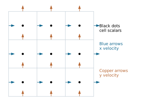
A Cartesian staggered grid stores scalars at cell centers and velocity components on faces normal to their axes. Harlow and Welch’s marker-and-cell formulation is the historical foundation [S2]. Pressure has $n_xn_yn_z$ entries; x-velocity has $(n_x+1)n_yn_z$, y-velocity has $n_x(n_y+1)n_z$, and z-velocity has $n_xn_y(n_z+1)$. These shapes differ even in a cubic domain.

With origin $\mathbf o$ and spacing $h$, a cell center is $\mathbf o+h(i+1/2,j+1/2,k+1/2)$. An x-face is at $\mathbf o+h(i,j+1/2,k+1/2)$. Each component therefore requires its own sampling offset. Using cell-centered offsets for all components creates a half-cell error and can destroy an otherwise correct projection.

Divergence from flux balance

Integrate divergence over a cubic cell, approximate each face flux by its stored normal velocity, and divide by volume:

$$(D\mathbf u)_{ijk}= \frac{u_{i+1,j,k}-u_{i,j,k}}{h} +\frac{v_{i,j+1,k}-v_{i,j,k}}{h} +\frac{w_{i,j,k+1}-w_{i,j,k}}{h}.$$

The pressure gradient at an interior x-face is $(p_{i,j,k}-p_{i-1,j,k})/h$. The same face appears in two neighboring divergences with opposite signs. This shared-face requirement gives cancellation of internal fluxes.

For the formal model, define a cells-by-faces matrix $B$. Each oriented internal face column contains $-1$ at its tail and $+1$ at its head. At unit spacing, physical divergence is $-B\mathbf u$, while pressure difference is $B^Tp$. The proofs and experiments use this convention. A uniform physical grid inserts factors $1/h$. Cut cells require cell-volume and face-area metrics, not an informal reuse of the unweighted identity.

The adjoint identity

Exchange finite sums:

$$\sum_i p_i\sum_e B_{ie}u_e =\sum_e\left(\sum_iB_{ie}p_i\right)u_e.$$

This exact discrete integration-by-parts identity says $p^TBu=(B^Tp)^Tu$. Physical divergence and gradient are negative adjoints. The Lean theorem named adjoint_identity proves the finite-sum statement for every real matrix of the declared shape. It does not prove that array traversal assembled the right matrix.

Two cells connected by one face give

$$B=\begin{bmatrix}-1\\1\end{bmatrix}, \qquad B^Tp=p_1-p_0, \qquad BB^T=\begin{bmatrix}1&-1\\-1&1\end{bmatrix}.$$

Face velocity 3 gives physical divergence $(3,-3)$, whose sum vanishes. Reversing both orientation and stored velocity sign preserves the physical field; reversing only one is a bug.

Layout and indexing

Use x-fastest flattening:

$$\operatorname{index}(i,j,k)=i+n_x(j+n_yk).$$

The Lean theorem flatten_in_bounds proves this lies below $n_xn_yn_z$ for in-range natural coordinates. Machine integers add a separate obligation: shape products and additions must fit before allocation or indexing. Validate shape arithmetic with checked operations when constructing the grid. Retain distinct validated shape types for cells and each face orientation. Repeated handwritten dimension arithmetic spreads the contract across every kernel.

Separate interior stencil loops from boundary updates. Ghost layers simplify sampling but enlarge storage and need one refresh owner. Stale ghost velocities can make transport and pressure use different wall conditions. Tests should include a constant field, linear pressure ramp, one nonzero face and manufactured divergence-free vortex, checking boundaries as well as interiors.

Rectangular cells and physical units

Let cell widths be $h_x,h_y,h_z$, volume $V=h_xh_yh_z$, and x-face area $S_x=h_yh_z$. Integrating mass flux first, then dividing by volume, gives $S_x/V=1/h_x$. Thus the rectangular-grid divergence has different denominators per direction. Replacing all three by one average spacing changes both the PDE and the pressure spectrum.

Pressure in pascals divided by x-center separation $h_x$ gives a pressure gradient in pascals per metre. Multiplying by inverse density and time step gives metres per second, as needed for a velocity correction. The x-face correction is

$$u^+_{i,j,k}=u^*_{i,j,k} -\frac{\Delta t}{\rho_{i,j,k}^{x}h_x} (p_{i,j,k}-p_{i-1,j,k}).$$

Substituting all three face corrections into divergence gives the familiar seven-point operator. With constant density, an interior row has diagonal $2/(\rho h_x^2)+2/(\rho h_y^2)+2/(\rho h_z^2)$, and opposite-direction neighbors receive the corresponding negatives. Every coefficient has units inverse density per square metre. The right-hand side is negative physical divergence divided by time step.

This row-divided form is symmetric when all volumes are equal. For unequal cell volumes, dividing each row by its own volume usually destroys Euclidean symmetry. CG must then use a symmetrized integrated system or a correctly weighted formulation. Calling the nonsymmetric row-divided matrix a Laplacian does not make ordinary CG valid.

Integrated metric construction

Separate topology from geometry. Let B be the unscaled incidence matrix, S the diagonal open-face area matrix, L the diagonal pressure-center distance matrix, and V the diagonal cell-volume matrix. Unknown face speed is u. Let Q be the vector of known outward volume flux through prescribed-velocity boundaries. Then

$$D u=V^{-1}(Q-BSu),\qquad G p=L^{-1}B^Tp.$$

The first expression is affine because of known boundary flux. The two-point gradient assumes pressure sample separation is aligned with the face normal and L contains that normal separation. This holds for the selected Cartesian MAC pressure sample locations. Positive areas, distances and volumes alone do not establish consistency for arbitrary cut-cell centroids. Nonorthogonal centroid corrections require a separately derived gradient and matching adjoint operator; they are outside this baseline. An affine-pressure fixture independently checks the normal-gradient consistency and demonstrates failure on a skew connection. With diagonal face density R, correction is $u^+=u^*-\Delta t R^{-1}Gp$. The symmetric integrated pressure system is

$$Kp=b,\qquad K=BSR^{-1}L^{-1}B^T, \qquad b=(BSu^*-Q)/\Delta t.$$

For positive geometry and density, face coefficient $S_e/(\rho_e\ell_e)$ is nonnegative. K has the same graph energy structure as the Lean model. It is symmetric in the ordinary Euclidean inner product because cell-volume division was left outside the solve. The physical residual relation is now

$$D u^+=-\Delta t\,V^{-1}(b-Kp).$$

Consequently a small integrated residual can still produce large divergence in tiny cells. A stopping test should inspect volume-scaled divergence as well as solver norms. The existing Lean theorem is the unweighted algebraic core; this physical metric interpretation is a derived specification.

For dimensional checking, $S/(\rho\ell)$ has units metres to the fourth per kilogram. Multiplying by pressure gives cubic metres per second squared, matching volume flux divided by time. V then converts the corrected flux mismatch to inverse seconds. This check catches missing density, distance and volume factors before a simulation is run.

Coefficient storage

For a regular rectangular grid, store dimensions and three reciprocal spacings once. For irregular geometry, each active face needs open area, pressure distance and density information, or a precomputed transmissibility with provenance. One transmissibility value must be shared by both adjacent pressure rows. Independently computing it twice can introduce asymmetry through different clipping or density choices.

At a density discontinuity, derive the coefficient from the selected pressure-gradient model. For two segments with lengths $\ell_a,\ell_b$ and densities $\rho_a,\rho_b$, a series-resistance argument gives transmissibility $S/(\rho_a\ell_a+\rho_b\ell_b)$. This differs from blindly averaging inverse density at the face. The correct choice depends on how pressure and acceleration are integrated; retain the derivation and test a one-dimensional interface fixture.

Cell-volume, face-area and center-distance validity are separate checks. A positive volume does not imply a valid connecting face. A zero area removes a connection; a zero distance is invalid. These distinctions determine graph connectivity and pressure gauges.