9 Liquid interfaces and volume

A liquid needs an interface representation beyond velocity. A level set stores $\phi$ , negative inside, with zero contour at the surface. A signed-distance field has $|\nabla\phi|=1$ nearby. Osher and Sethian introduced a Hamilton-Jacobi framework for evolving fronts [S8]. Merging and splitting are natural, but interpolation and reinitialization can move the contour.

Reinitialization

Transport satisfies $\partial_t\phi+\mathbf u\cdot\nabla\phi=0$ . A common distance-restoring evolution is

$\partial_\tau\phi+ \operatorname{sgn}(\phi_0)(|\nabla\phi|-1)=0.$

Artificial time $\tau$ seeks distance-like values with fixed reference sign. Discretization can shift the zero set, especially in thin sheets. Reinitialization frequency, stencil, sign smoothing and termination belong to the method specification. Smooth appearance does not imply correct volume.

A narrow band must cover interpolation support and travel before rebuilding. Outside values need valid classification and reconstruction when activated. Invalid far-field sentinels must not be interpolated into the surface.

Pressure at the free surface

Neglecting air dynamics, surface tension and liquid normal viscous stress, set surface pressure to atmospheric zero. If normal viscous stress is retained, this is only a declared split approximation; a coupled traction condition is required as discussed in Chapter 10 and Batty-Bridson Section 3 [S11]. A pressure connection with interface distance $\alpha h$ uses that shorter distance, increasing its coefficient as $\alpha$ shrinks. A minimum-distance policy changes pressure and interface error and must be evaluated.

Velocity needs extension into a limited air band for transport. The pressure-unknown mask, velocity-validity mask and distance-band mask are distinct. Extending velocity does not mean the whole air region solves the liquid equations.

Volume fractions

A fraction $f_i\in[0,1]$ gives represented volume

$V_h=\sum_i f_iV_i.$

Shared liquid-volume fluxes with opposite signs preserve global volume except for sources and boundaries. Hirt and Nichols established the volume-of-fluid approach [S9]. Geometric reconstruction estimates a local interface to determine swept liquid volume; it is substantially more work than advecting a color scalar.

A cell fraction 0.3 and Courant number 0.5 illustrate the risk: an outgoing flux selected without interface geometry can remove more liquid than exists. Bounding available volume must coordinate faces in multiple dimensions. Clamping final fractions can restore range while destroying total volume. Preserve both by construction or disclose the correction.

Particle correction and extraction

Particle level-set methods use particles carrying side-of-interface information to correct local errors [S10]. Reseeding, radii and collision handling add state and memory. They do not make level-set volume exact.

Select a liquid method from acceptance metrics. Level sets simplify smooth geometry but need drift budgets. Volume fractions expose conservation but need reconstruction. Hybrids increase verification burden. Finish the baseline grid contracts before committing to a liquid branch.

Mesh extraction adds its own error. Edge crossings and ambiguous cases need consistent rules across cells. Normals use physical spacing and safe treatment of small gradients. Validate spheres at several subcell offsets, thin sheets and merging components. Compare volume, surface distance and rasterized silhouette separately. A guidance mesh need not be manufacturing-grade, but its promised topology must be explicit.

Piecewise linear interface reconstruction

A volume-fraction method needs geometry inside partially filled cells. A piecewise linear interface reconstruction chooses a unit normal n and plane offset d so the liquid region inside a cell is $\{x:n\cdot x\leq d\}$ and its volume matches $f_iV_i$ . For this liquid-side inequality, outward n is minus the normalized fraction gradient, since f decreases toward air. For a negative-inside level set, outward n is plus the normalized phi gradient. Use a resolved neighborhood estimate; when its norm is too small, return an unresolved normal or use a documented geometry-derived fallback, never normalize zero. The offset fraction-step fixture checks both signs. Then solve for d by a monotone volume function.

On a unit cube with n along positive x, the solution is simply $d=f_i$ for fractions in $[0,1]$ . For a general normal, clip the cube polyhedron against the plane and compute its volume, or use a verified analytic formula. Bisection is robust because volume increases monotonically with d. Bracket d using the minimum and maximum plane projections of cube vertices. Stop according to volume and geometric tolerances, not an arbitrary iteration count alone.

Transport then clips the reconstructed liquid region against the swept face volume over the step. In a simple axis-aligned constant-speed case, this is a slab of width $u\Delta t$ . In multiple dimensions, directional splitting and unsplit flux constructions handle corner transport differently. A raw sum of independently computed face outflows can exceed available liquid. A production implementation must select one coherent bounded-conservative method and test its multidimensional flux accounting.

The expanded companion only checks the axis-aligned slab case: a cell filled to fraction 0.3 with a positive swept width 0.5 sends the geometrically intersected amount under an explicitly positioned interface. It does not claim a complete arbitrary-normal PLIC implementation. General polyhedral clipping, orientation robustness and multidimensional boundedness remain implementation work.

Curvature from a level set

With outward normal $\mathbf n=\nabla\phi/|\nabla\phi|$ , mean-curvature sum is $\kappa=\nabla\cdot\mathbf n$ . In three dimensions a sphere of radius R has $\kappa=2/R$ under this convention. When air viscous stress is negligible, normal traction balance is $p_{\mathrm{liquid}}-p_{\mathrm{air}}=\sigma\kappa+\mathbf n^T\tau_{\mathrm{liquid}}\mathbf n$ . The simpler Laplace jump $\sigma\kappa$ additionally neglects normal liquid viscous stress. Tangential traction still requires its own condition. See Chapter 10 and [S11] Section 3; a pressure-only split must declare its approximation. Reversing the sign convention for phi reverses normal and curvature, so the pressure-jump sign must change consistently.

A direct finite-difference curvature formula is

$\kappa= \frac{|\nabla\phi|^2\operatorname{tr}(H_\phi) -(\nabla\phi)^TH_\phi\nabla\phi} {|\nabla\phi|^3}.$

It requires first and second derivatives and becomes ill-conditioned when gradient magnitude is small. Regularizing the denominator changes the curvature estimate. Near underresolved sheets or merged surfaces, a smooth signed-distance assumption may fail even if every value is finite.

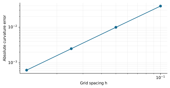
The companion evaluates a sphere distance field and central-difference curvature at a known surface point over decreasing h. It compares against $2/R$ . This is a derivative-stencil fixture, not a moving-droplet surface-tension validation. Production tests must additionally measure parasitic currents in a stationary droplet, pressure jump and oscillation behavior.

Surface tension time scales

Balance capillary pressure $\sigma/h$ against inertial acceleration over length h. Acceleration scale is $\sigma/(\rho h^2)$ ; moving distance h under that acceleration gives time scale $\sqrt{\rho h^3/\sigma}$ . This dimensional derivation explains severe restrictions as resolution increases. The stability constant depends on the actual discretization and integration method.

For a 1 cm feature scale, density 1000 kg per cubic metre and surface tension 0.072 newtons per metre, the dimensional time scale is approximately 0.118 seconds. At a 1 mm scale it is about 0.00373 seconds. These are scale estimates, not accepted time-step limits for an unimplemented solver.

Implicit tension may relax a stability restriction but introduces coupled geometry or linearization errors. It does not eliminate the need to resolve curvature or validate the interface. Likewise, increasing surface tension to suppress noise changes the material and can alter the desired guidance shape.

Volume correction as a declared operation

A level-set volume correction sometimes shifts phi by a constant until a target volume is restored. This moves the interface everywhere, including regions already accurate. It can repair a scalar volume metric while damaging local positional accuracy. If used, record shift magnitude, affected volume and resulting silhouette displacement.

A more informative acceptance report retains both volume drift and a spatial surface metric. Two shapes can have equal volume and completely different placement. Rheon’s guidance purpose makes that distinction especially important.

A shared-face experiment

Start with one unit-metre cube and an empty receiving cube. Prescribe positive x transport over one interval, with swept width $c=u\Delta t/h$ between zero and one. The outgoing region is $[1-c,1]\times[0,1]^2$ . The interface position, not just the liquid fraction, determines how much liquid intersects this slab.

The embedded example places the same fraction $f$ in either $[0,f]\times[0,1]^2$ or $[1-f,1]\times[0,1]^2$ . The two transferred volumes, in cubic metres for these unit cubes, are

$Q_L=\max(0,f+c-1),\qquad Q_R=\min(f,c).$

Predict before switching Liquid location: with $f=0.3$ and $c=0.5$ , the left-filled cell transfers zero, while the right-filled cell transfers 0.3 m³. A uniform-mixture estimate $cf=0.15$ cannot distinguish these interfaces. It can preserve a shared ledger while giving a different interface transport. Teal marks the initial liquid, orange the swept region, and the dark intersection the outgoing liquid. Orbit the cube to inspect their spatial relationship. Lower cubes encode the resulting amounts with fill heights; they do not claim reconstructed post-step geometry.

The receiver starts empty. Subtract the same Q from the donor and add it to the receiver: $(f-Q)+Q=f$ . Now inspect the deliberately incorrect full-slab transfer $Q=c$ : the amounts become −0.2 and 0.5 m³. Independently clamping them gives zero and 0.5 m³, creating 0.2 m³. Conservation, bounded fractions and geometrically correct transport are three separate questions.

This is a one-face geometric/ledger experiment, not a closed-box divergence-free velocity solution. Two liquid-containing cells, several outgoing faces, inflow, non-unit cell volumes and arbitrary normals require additional accounting. The receiver’s capacity must also be respected. Slider width up to one is an intersection domain, not a stability recommendation for a multidimensional scheme.

Research connection and native scope

The official Basilisk VOF implementation reconstructs a plane before evaluating liquid in a swept face region. Its one-dimensional sweep includes a compression contribution; the multidimensional construction follows Weymouth and Yue’s conservation treatment and states an exactly non-divergent velocity condition. Its documented CFL restriction is 0.5. These details explain why isolated face cancellation does not establish bounded, conservative multidimensional VOF. See its sweep_x and vof_advection implementations (consulted 2026-10-13), alongside Hirt and Nichols [S9]. This lesson implements neither complete scheme.

Rheon’s existing liquid-volume owner and liquid step remain separate native code. This browser lesson does not invoke them, change their admission rules, or qualify geometric reconstruction in Rust. Its independent equations are visible in volume_reference.js.

Checked volume-flux proof bridge

VolumeFlux.lean states exact-real properties with explicit hypotheses. For $0\le f,c\le1$ , the left slab flux is nonnegative and no greater than either f or c. The right slab has the same bounds under nonnegative f and c. A shared transfer cancels from the combined ledger for any real donor, receiver and transfer amount. Bounded post-transfer amounts additionally require a nonnegative transfer, sufficient donor availability, donor amount at most one, nonnegative receiver amount and receiver capacity. Exact rational witnesses distinguish the two placements and show clamping’s 0.2 m³ volume creation.

These statements do not prove that JavaScript implements the geometry, that IEEE arithmetic is exact, or that the native liquid algorithm converges. The source inventory and kernel qualification status are recorded separately in the coverage ledger; numerical comparisons and browser control checks supply different evidence. Proof text is collapsed by default in the interactive chapter.

Original reference illustration for 9 Liquid interfaces and volume