23 Wetting, adhesion and the contact line

Wetting describes a liquid’s preference for solid contact in relation to surrounding phases. Adhesion names interfacial energetic attraction; slip describes tangential motion; viscosity describes bulk stress. These are not interchangeable controls. A liquid can have a small equilibrium contact angle and substantial slip, or a large angle with strong viscous drag. A wall that numerically pins every trace can look sticky without implementing an adhesion model.

Equilibrium surface energy

For a smooth homogeneous ideal solid, write interfacial energies $\gamma_{sv}$, $\gamma_{sl}$ and liquid-vapor tension $\sigma>0$, all in N/m. The equilibrium Young relation is

$$\gamma_{sv}-\gamma_{sl}=\sigma\cos\theta_e.$$

The reversible work of adhesion is $W_A=\gamma_{sv}+\sigma-\gamma_{sl}$, giving $W_A=\sigma(1+\cos\theta_e)$. young_adhesion_identity proves this implication from a stated algebraic Young balance. adhesion_bounds assumes a cosine value in [-1,1] and proves $0\leq W_A\leq2\sigma$. These are energetic identities, not a microscopic derivation, an existence theorem for a droplet, or a proof of dynamic contact angle.

Only the difference of solid interfacial energies is inferred by an angle. Their individual values remain unidentified. Nor does $W_A$ specify a bulk attractive body force. Adding an arbitrary wall attraction while also imposing the same contact angle can count energetic effects twice. A chosen disjoining-pressure or precursor-film model requires its own potential, length scale and calibration.

Constant-volume cap geometry

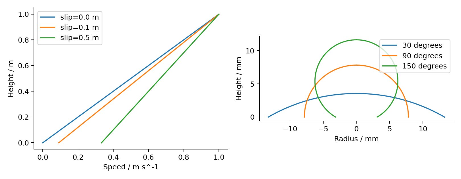
In negligible gravity, an axisymmetric spherical cap with curvature radius R has height $H=R(1-\cos\theta)$, contact radius $a=R\sin\theta$, and volume

$$V=\tfrac\pi3R^3(2-3\cos\theta+\cos^3\theta).$$

For fixed V, solve this equation for R before changing angle. Drawing every cap with the same sphere radius changes liquid volume and confounds the demonstration. The original fixture holds V at $10^{-6}$ m³, samples angles from 30 to 150 degrees, and independently integrates circular cross sections to check volume. All cap meshes, pressure jumps and adhesion readouts use these same stored records.

Basilisk’s original 3D sessile-drop test provides a primary implementation and analytic comparison [E6]. The present cap lab evaluates analytic equilibrium geometry; it does not simulate relaxation. Density and viscosity therefore do not affect its equilibrium shape. Gravity and finite Bond number invalidate this spherical-cap oracle.

Contact-angle reconstruction

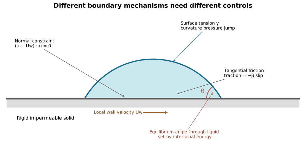
A negative-inside level set gives an outward liquid normal. Let the solid normal point into the accessible fluid. At a flat horizontal solid, the cap’s liquid normal obeys $n_l\cdot n_s=\cos\theta$. Curved or angled surfaces require a local wall frame and a contact-line tangent. A two-dimensional ghost slope copied directly into three dimensions can impose the wrong angle.

Afkhami and Bussmann’s original height-function method accounts for the orientation of the contact-line projection in 3D [E7]. Its geometry and refinement results are method-specific. Basilisk’s documented contact implementation includes restrictions at shallow angles and unresolved height support [E8]. Rheon’s proposed admission rule reports unresolved normals rather than advertising all-angle accuracy.

Dynamics and hysteresis

A sharp moving contact line with strict no-slip has a classical stress-singularity difficulty. Cox’s original analysis addresses a small-capillary-number regime with a microscopic slip or other regularization scale [E9]. A static angle alone is not a complete dynamic law. A proposed model must identify microscopic regularization, apparent-angle observation scale and contact-line mobility.

Advancing and receding angles can define a pinned interval with motion outside it. That is an additional hysteresis model, not an automatic consequence of Young’s relation. Heterogeneous solids, roughness and contamination can change observed behavior. Start with a declared smooth equilibrium model, then qualify contact-line speed, angle and volume under refinement before adding hysteresis. No such dynamic contact-line solver is implemented or formally verified by this edition.

Moving contact lines

A static angle closes an equilibrium geometry problem. It does not determine how a contact line moves. Huh and Scriven’s original creeping-flow analysis shows the divergent stress and dissipation associated with a sharp moving contact line under the classical adherence condition. A finite grid may conceal the singularity by supplying numerical slip; refining that grid changes the concealed length scale. R04

Choose and state one regularization:

• Resolve a physical or effective Navier slip length and a compatible dynamic contact-angle closure.
• Use a diffuse interface with specified interface thickness, mobility, wall free energy, and wall relaxation law.
• Use a precursor-film/disjoining-pressure model with its own microscopic length scale.
• Pair an explicitly labeled engineering angle-speed law with effective slip, diffusion or another declared microscopic cutoff. Advancing/receding limits and pinning are optional additional models; the angle-speed law alone does not remove the sharp no-slip singularity.

For a low-capillary-number hydrodynamic approximation, the familiar small-angle form is

$$\theta_{app}^{3}-\theta_{micro}^{3} \simeq 9\,Ca\log(L/\ell_{micro}),\qquad Ca=\mu U_{cl}/\gamma.$$

Here Ucl is signed, the angle is in radians, and L is the stated observation scale. This expression is not a universal all-angle, high-speed law. The general Cox construction concerns small Ca, scale separation, and a two-fluid viscosity ratio; at finite gas viscosity the full angle function replaces the cubic shorthand. Use the expression as a labeled asymptotic comparison only within those assumptions. R05

Qian, Wang, and Sheng combine Cahn–Hilliard interfacial free energy with a generalized Navier boundary condition containing uncompensated Young stress. They compare the continuum model with molecular-dynamics profiles, including Couette and Poiseuille configurations. That is stronger evidence than an attractive drop image, but it does not license transplanting their fitted molecular parameters to an arbitrary macroscopic liquid or treating diffuse-interface mobility as a harmless numerical knob. R06

For contact-angle hysteresis, an engineering pinned state may allow θR ≤ θapp ≤ θA with Ucl = 0. An advancing or receding branch applies outside that interval. Store θR, θA, the observation scale, and the dynamic law separately. Static friction, capillary pinning, and high bulk viscosity can all delay motion while representing different physics.

Partial wetting has an admissible range

Young balance requires σ>0 and |(γsv−γsl)/σ|≤1. Outside that interval, clamping the inferred cosine hides a changed model. The spreading coefficient S=γsv−γsl−σ distinguishes the ideal complete-wetting tendency when S≥0; a precursor film or disjoining pressure then needs extra length scales. The fixed-volume cap reference deliberately stays within partial wetting and does not provide a film model.

With fixed total solid area, surface energy can be written E_s=σ(A_lv−cosθ_e A_sl) up to a constant. Changing μ changes the relaxation path, while changing θ_e changes this ideal energy landscape. A nearly stationary highly viscous drop may be far from equilibrium. An empirical SPH cohesion/adhesion force is a possible visual model R11, but its coefficient is not automatically the gradient of this area energy or a calibrated interfacial tension.