5 Solving the pressure system

Pressure often determines both frame cost and volume quality. The solver receives an SPD reduced system or an explicitly handled semidefinite system. It returns pressure, iterations, true residual, termination reason and breakdown diagnostics. A vector alone loses information needed to accept or reject a frame.

Jacobi as a reference

With diagonal $D_A$, weighted Jacobi is

$$p^{k+1}=p^k+\omega D_A^{-1}(b-Ap^k).$$

Convergence requires spectral radius below one for $I-\omega D_A^{-1}A$ on the solved subspace. Parallel local access is simple, but smooth error can decay slowly as grids grow. A fixed iteration count is not fixed divergence quality. Isolated zero-diagonal cells must be classified, never divided by zero.

Jacobi is useful as an independent reference and multigrid smoother. Compare time to an accepted residual, including reductions and synchronization, not one iteration against an unrelated solver iteration.

Conjugate gradients

For an SPD matrix and SPD preconditioner $M$, initialize $r_0=b-Ap_0$, $z_0=M^{-1}r_0$, $d_0=z_0$. Then

$$\alpha_k=\frac{r_k^Tz_k}{d_k^TAd_k},\quad p_{k+1}=p_k+\alpha_kd_k,\quad r_{k+1}=r_k-\alpha_kAd_k,$$

$$z_{k+1}=M^{-1}r_{k+1},\quad \beta_k=\frac{r_{k+1}^Tz_{k+1}}{r_k^Tz_k},\quad d_{k+1}=z_{k+1}+\beta_kd_k.$$

Shewchuk develops Krylov methods and conditioning in detail [S5]. Rheon’s operational contract additionally detects nonfinite values, nonpositive curvature, zero denominators and exhausted budgets. Check the initial residual before forming any quotient. Zero right-hand side and zero guess should return immediately.

The exact-arithmetic energy-error bound for SPD systems is

$$\|e_k\|_A\leq 2\left(\frac{\sqrt\kappa-1}{\sqrt\kappa+1}\right)^k\|e_0\|_A.$$

It is not a runtime prediction. Spectrum, preconditioner cost, precision and memory traffic matter; a singular system requires a specified subspace. The current Lean package does not prove CG convergence.

Preconditioner selection

Diagonal scaling is cheap and parallel. Incomplete Cholesky can reduce iterations but adds factorization, ordering dependence and triangular solves. Modified incomplete Cholesky is discussed in Bridson’s notes [S4]. Geometric multigrid attacks smooth error, but coarse levels must retain obstacle and free-surface semantics. A coarse operator that reconnects sealed regions changes the nullspace.

A matrix-free seven-point stencil is attractive for a known regular coefficient structure. Reconstruct neighbor contributions from face weights and diagonals. An explicit sparse matrix remains valuable in tests as an inspectable independent oracle. Comparing two wrappers around one kernel cannot catch shared assembly errors.

Residual and warm starts

Recursive residuals drift from $b-Ap$ in floating point. Recompute the true residual at termination and periodically where needed. Document direction restarts after replacement. Warm starts help only when operator, pressure gauge and topology remain compatible. New disconnected components or grid rescaling require remapping or reset.

The companion uses an 8-cubed closed grid, removes one row and column, and projects deterministic random velocity. It records CG and weighted-Jacobi histories. This compares mechanisms on that small system, not production frame time. Failure leaves the last accepted state intact or publishes a declared degraded preview according to an explicit lifecycle policy.

Residual scales and breakdown policy

Let the integrated solve be $Kp=b$. A relative criterion $\|r\|_2\leq\tau_{\mathrm{rel}}\|b\|_2$ can be combined with an absolute criterion, but physical acceptance is additionally $\|\Delta t V^{-1}r\|_\infty\leq\tau_{\mathrm{div}}$. The first measures linear-system progress; the second limits maximum cell divergence. They can disagree in cut cells. Physical acceptance must reconstruct the full ungauged residual on every active cell, including eliminated gauge cells. A reduced-system residual alone can hide accumulated imbalance in the removed row. Independently recompute divergence on every active cell after correction. The companion includes a compatible chain where all retained residual entries pass a threshold but the eliminated row fails it.

For a diagonal preconditioner, require positive diagonal entries for every reduced unknown. If the matrix has a zero row, classify the topology before invoking CG. If $r^Tz$ or $d^TKd$ is nonpositive in an expected SPD solve, return a breakdown with the iteration and scalar values. Do not take an absolute value or clamp the denominator; that changes the method and conceals the failed assumption.

The source of a breakdown can be an invalid operator, wrong gauge, loss of precision or an inappropriate preconditioner. Retrying in higher precision is useful only after the operator checks pass. A retry should start from a coherent state, recompute true residual and retain the original failure diagnostic.

Why multigrid helps

Jacobi damps different error frequencies at different rates. For a one-dimensional uniform Dirichlet Laplacian, the diagonal-scaled Fourier symbol is $1-\cos\theta$. Weighted Jacobi’s error multiplier is $1-\omega(1-\cos\theta)$. Small $\theta$ gives a multiplier near one, so smooth error decays slowly. After transferring to a coarser grid, that same physical error becomes less smooth in grid coordinates and easier to correct.

This argument motivates a two-grid method: smooth the current estimate, restrict its residual, solve for a coarse correction, prolong it, and smooth again. Saad provides a primary textbook treatment of multigrid and sparse iterative methods [S22]. The construction below states Rheon’s proposed contract rather than asserting an implemented hierarchy.

Transfer operators

Let P map coarse pressure corrections to fine pressure corrections. For uniform cell-centered grids, construct P by trilinear interpolation at fine cell centers expressed in coarse-cell coordinates. The offset is important: a fine center is not generally a coarse node. Near boundaries, interpolation must respect prescribed pressure and component membership.

Choose restriction R consistently with the inner product. In an integrated symmetric system, $R=P^T$ yields the Galerkin operator $K_H=P^TK_hP$. If $K_h$ is SPD and P has full column rank on the solved subspace, then for nonzero coarse x,

$$x^TK_Hx=(Px)^TK_h(Px)>0.$$

Thus coarse SPD follows from construction, with explicit rank and subspace assumptions. For volume-normalized residuals, volume-weighted restriction is more natural; convert consistently instead of mixing formulas.

On a closed graph, preserving constants requires $P\mathbf1_H=\mathbf1_h$. Coarse connectivity must not join separate fine components. A coarse cell spanning a thin solid barrier needs multiple component degrees of freedom or a hierarchy policy that preserves separation. Otherwise the coarse correction allows nonphysical communication.

V cycle specification

v_cycle(level, rhs, estimate):
    if level is coarsest:
        solve the gauge-fixed coarse system accurately
        return estimate
    apply fixed pre-smoothing sweeps
    residual = rhs - K[level](estimate)
    coarse_rhs = transpose(P[level]) * residual
    coarse_error = zero
    coarse_error = v_cycle(level + 1, coarse_rhs, coarse_error)
    estimate += P[level] * coarse_error
    apply compatible post-smoothing sweeps
    return estimate

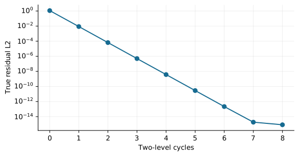
As a standalone solver, monitor the finest-grid true residual after cycles. As a CG preconditioner, the V cycle must act as a fixed linear SPD map on the relevant subspace. Matching adjoint pre/post smoothing and an SPD coarse solve are important. Adaptive iteration counts, nonsymmetric Gauss-Seidel order or changing hierarchy can violate the usual PCG assumptions. A flexible Krylov method is a different algorithmic choice, not a label to add after the fact.

The expanded companion constructs a small Dirichlet one-dimensional hierarchy with interpolation P, Galerkin coarse matrix and weighted Jacobi smoothing. It checks symmetry, positive eigenvalues and measured residual reduction. This is an executable mechanism fixture, not a three-dimensional obstacle-aware multigrid implementation.

Storage and work

A regular three-dimensional geometric hierarchy has cell counts $N,N/8,N/64,\ldots$; their sum approaches $8N/7$. This favorable count excludes per-level masks, transfer metadata, coefficients and temporary vectors. An irregular hierarchy can have much more overhead. Count actual simultaneous buffers, especially when used inside PCG.

For low-resolution Rheon scenes, a simpler diagonal-PCG solve may outperform a complex hierarchy once setup and changing geometry are included. Measure complete solve time to a physical tolerance. Multigrid is a promising mechanism, not a required optimization before evidence.

Draft checkpoint: qualify a model’s pressure before using it

Unmerged PR49, inspected at b8ca87cab7f74f64c1686714a33e843fbb178c3d, introduces an opt-in pressure-provider workspace. The native modal model evaluates a frozen learned transform/gain checkpoint in one fixed 32³ sealed unit box, with density 1.25 kg/m³ and dt = 1/60 s. The draft’s model provenance and qualification contract links the exact upstream source/checkpoint and separates its historical rollout measurements from this native pressure-stage experiment.

Predict the response when density or grid shape changes: the model declines and the matching numerical reference is used. For an admitted request, every output must be finite and gauge-consistent, and the workspace recomputes the full ungauged residual, including the gauge cell. A declined or rejected candidate uses a fresh zero-start numerical reference; cancellation aborts without fallback. The caller must still check divergence of its actual corrected f32 velocity before publication. Pressure acceptance alone is not a complete step contract.

The SHA256-verified export and trusted checkpoint supply artifact provenance; the loader’s FNV corruption check is not cryptographic authentication. Timing columns separate inference, qualification and fallback, while excluding model construction and caller velocity correction. Neither an accepted prediction nor a historical speed ratio establishes faster full trajectories, general physical accuracy, GPU support or arbitrary-geometry learning. Defaults and PR48’s transport facade are not automatically switched to this draft provider.

Two disconnected pressure regions

Start with two regions that cannot exchange fluid, each containing two cells. The embedded example recomputes an all-Neumann pressure correction with unit cross-section, density 1 kg/m³ and dt=1 s. Cell widths encode actual volumes. For volumes (1,3,2,2) m³, both centre distances are 2 m and both face weights are 1/2. Compatible integrated data b=(1,-1,2,-2) gives fixed-left pressures (0,-2,0,-4) Pa and internal velocity corrections (1,2) m/s.

Predict what adding the same pressure to both cells of region A will change. The scalar pressure bars move, but that region’s pressure difference and face correction do not. Bars use the display depth as a scalar axis; they are not force vectors. The separated boxes represent disconnected regions, not a fluid simulation with hidden exchange across the gap.

Global balance can hide component errors

Now select b=(1,0,-1,0). Its global sum is zero, but its two component sums are 1 and -1. The original equations cannot both be satisfied in either region. Fixing each left cell and solving only the right rows returns zero pressures. The retained-row residual is zero, yet the full residual is (1,0,-1,0) and actual divergence is (-1,0,1/2,0) /s. Read the rejected status before trusting a small reduced residual. A gauge cannot repair incompatible boundary data.

Fixed-cell and mean-zero gauges

For compatible data, fixing one pressure per region or subtracting each region’s arithmetic pressure mean changes only its representative. The pressures become (1,-1,2,-2) Pa with arithmetic means zero; the face corrections stay (1,2) m/s. Fixing one cell in the entire disconnected system is insufficient. These are algebraic gauges, not prescribed physical pressure boundaries.

Volume-weighted pressure gauges

A volume mean uses V-weighted pressure. For unequal cells it gives (3/2,-1/2,2,-2) Pa, which differs from the arithmetic mean while preserving all within-region pressure jumps. Minimum-norm language needs its inner product: Euclidean and volume-weighted norms choose different representatives. The offset controls deliberately shift away from the selected zero constraint for comparison. Pressure differences across independent regions remain undetermined here.

Projecting a source changes the problem

For incompatible b, the explicit projection comparison changes it to (1/2,-1/2,-1/2,1/2). That modified system has a solution. Its original-system residual is still (1/2,1/2,-1/2,-1/2), so the original boundary data remains rejected. The source-change readout is part of the result: projection is not a silent gauge choice or a physically justified repair.

Gauge shifts and boundary work

The outward-flux pairing includes external work:

$$p_L(q+Q_L)+p_R(-q+Q_R)=-(p_R-p_L)q+p_LQ_L+p_RQ_R.$$

A common shift c changes boundary work by c(Q_L+Q_R), while the internal term is unchanged. It vanishes for each balanced region. With incompatible data, region offsets (2,-2) Pa produce -4 W of boundary pairing even though the global flux sum is zero. This exposes inconsistent data, not an absolute-pressure prediction for a valid closed flow.

A pressure error is not a gauge

Perturb only the right pressure in region A by 1/4 Pa. Compatible unequal cells then have residual (1/8,-1/8,0,0), divergence (-1/8,1/24,0,0) /s and internal velocity correction 7/8 m/s in A. The physical pressure difference changed; zero total flux does not make this locally valid. This is an intentional finite perturbation, not a floating-point model.

Two unknowns and a real iteration

Use K = [[2, −1], [−1, 2]], corresponding to a two-cell Dirichlet stencil. From x = 0, each control-selected iteration performs x ← x + α(b−Kx)/2 using the complete old vector. This is simultaneous weighted Jacobi, rather than a saved-field blend. For b = (1, 0), the exact solution is (2/3, 1/3). At α = 1 after four iterations, x = (5/8, 5/16), the true residual is (1/16, 0), and error energy eᵀKe is 1/384. The readout recomputes b−Kx. At α = 1/2 with alternating b after eight iterations, each residual magnitude is 1/65536. Its fixed-scale arrow is nearly invisible; the numerical readout remains available. A minimum visible shaft would exaggerate that residual and violate the scale.

A positive matrix with an unstable iteration

The matrix energy is (x−y)² + x² + y² and is positive away from zero. Smooth and alternating error modes nevertheless have iteration factors 1−α/2 and 1−3α/2. Both contract only when 0 < α < 4/3. Select α = 3/2 and alternating b: the alternating error factor is −5/4 and its energy grows by 25/16 each iteration. Matrix positivity alone does not choose a stable Jacobi relaxation. Shewchuk, sections 5.2–5.3 explains the splitting and spectral-radius criterion; this matrix and its closed-form error modes are independently derived here. Production Krylov methods additionally need suitable operator/preconditioner properties and fresh full residuals; no general CG or multigrid result is inferred.