6 Transport and the price of stability

A passive scalar satisfies $\partial_tq+\mathbf u\cdot\nabla q=0$ for incompressible source-free flow. Along an exact characteristic it is constant. Semi-Lagrangian transport traces backward from an arrival sample and interpolates the old field. Stam’s stable-fluids construction popularized this in interactive graphics [S1]. Stability must name a norm and interpolation rule.

Backtracing

First-order tracing uses $\mathbf x_d=\mathbf x-\Delta t\mathbf u(\mathbf x)$. A midpoint estimate first samples velocity halfway along that estimate, then traces with the midpoint velocity. Each staggered component uses its own lattice offset; the scalar has another offset.

Trilinear interpolation is a convex combination of eight values when fractional coordinates lie in $[0,1]$. Nonnegative weights summing to one give

$$\min_iq_i\leq\sum_iw_iq_i\leq\max_iq_i.$$

Convex_sum_bounds proves this finite real statement. Repeated bounded interpolation cannot leave the original global range if boundaries and sources obey it. This does not imply conservation of all sample values.

Row sums and column sums

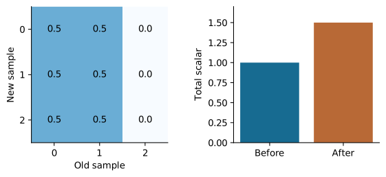
For $q^{+}=Tq$, convex interpolation means nonnegative entries and unit row sums. Conservation of an unweighted total requires unit column sums. For example,

$$T=\begin{bmatrix}1/2&1/2&0\\1/2&1/2&0\\1/2&1/2&0\end{bmatrix}$$

maps $(1,0,0)$ to $(1/2,1/2,1/2)$. Outputs are bounded but total rises from 1 to 1.5. The exact rational arithmetic is checked in Lean. This is a matrix counterexample to an implication, not a claim that this matrix comes from smooth incompressible periodic flow.

Constant translation on a periodic uniform one-dimensional grid happens to give a doubly stochastic interpolation matrix. The companion’s box test verifies that special case, not general semi-Lagrangian conservation. Variable velocity and irregular boundaries need separate evidence.

Numerical diffusion

For positive constant speed and Courant number $c=u\Delta t/h$ in $[0,1]$,

$$q_j^{+}=(1-c)q_j+cq_{j-1}.$$

A Fourier mode has amplification $g=(1-c)+ce^{-\mathrm i\theta}$, hence

$$|g|^2=1-2c(1-c)(1-\cos\theta).$$

Amplitude generally decays. Taylor expansion gives leading artificial diffusion $uh(1-c)/2$ under fixed-Courant refinement. A bounded solver can therefore erase thin jets or smear silhouettes. Arbitrarily large stable steps also degrade trajectory accuracy and obstacle interaction.

Conservative flux updates

Finite volume computes one shared face flux and applies opposite signs:

$$q_j^{+}=q_j-\frac{\Delta t}{h} (F_{j+1/2}-F_{j-1/2}).$$

Summation over periodic cells cancels all internal fluxes. Positive-speed upwind flux $F_{j+1/2}=uq_j$ preserves positivity for $0\leq c\leq1$, proved by upwind_positive. At $c=3/2$, $q_j=1$, $q_{j-1}=0$, the new value is $-1/2$, also formally checked. Conservation does not imply positivity.

The field determines the contract. A smoke appearance tracer may tolerate measured dissipation. A liquid fraction needs bounded conservative transport and interface geometry. A signed-distance field needs surface-position analysis. One generic quality parameter cannot hide these differences.

Component aware trilinear sampling

For an x-face field, convert world position to lattice coordinates $s=((x-o_x)/h_x,(y-o_y)/h_y-1/2,(z-o_z)/h_z-1/2)$. For a y-face, subtract half from x and z; for a z-face, subtract half from x and y. For cell-centered scalars subtract half from all coordinates.

Let $a=\lfloor s\rfloor$ and $t=s-a$. The eight weights are products of either $t_d$ or $1-t_d$. For corner $\epsilon\in\{0,1\}^3$,

$$w_\epsilon=\prod_{d=1}^3 \bigl(\epsilon_dt_d+(1-\epsilon_d)(1-t_d)\bigr).$$

Their sum factors into $\prod_d(t_d+1-t_d)=1$. Nonnegativity follows when each fractional coordinate lies in $[0,1]$. This derivation explains the exact hypotheses of the interpolation proof. Boundary remapping must preserve or deliberately replace the stencil; simply dropping invalid corners breaks partition of unity.

An affine scalar $q(x,y,z)=a+bx+cy+dz$ is reproduced exactly by trilinear interpolation on a complete stencil in real arithmetic. The expanded companion tests this on all four lattice offsets using independently evaluated world positions. It then deliberately uses the wrong offset for an x-face field to show the expected half-cell bias. This fixture catches a defect that constant-preservation tests miss.

Sampling boundaries

Periodic sampling wraps integer indices modulo the component’s periodic extent, accounting for duplicated boundary faces if the storage convention has them. A closed-wall sampler uses its declared ghost extension. A clamped texture sampler repeats edge values; it is not automatically a no-slip boundary condition. An out-of-domain trace at an open boundary needs a prescribed exterior value or a validity failure.

Return a sample together with validity information when the method needs it. Corrected advection needs to know whether forward and reverse stencils are valid and reversible. A scalar value alone cannot communicate that a trace hit a wall or crossed a source discontinuity.

Trace integrators

For an autonomous frozen velocity field, midpoint backtracing is

$$k_1=\mathbf u(\mathbf x),\quad k_2=\mathbf u(\mathbf x-\tfrac12\Delta t k_1),\quad \mathbf x_d=\mathbf x-\Delta t k_2.$$

A higher-order trace reduces ODE integration error but cannot improve interpolation order or unresolved velocity detail. For time-varying velocity, temporal interpolation between known levels is another approximation. Name which field drives tracing: old velocity, provisional velocity or projected velocity. These choices change the splitting.

A solid-rotation fixture with $\mathbf u=(-\omega y,\omega x,0)$ has an analytic rotation trajectory. Compare departure points against the exact rotation over one step and over one period. A translation fixture cannot distinguish Euler from midpoint tracing because both are exact for constant velocity. The companion includes the rotation test specifically to expose that difference.

Failure fixtures

Use a constant field to test partition of unity, an affine field to test offsets, a sinusoid to measure dissipation, a top-hat to reveal overshoot and limiter behavior, and a segment crossing a thin wall to test collision handling. Add a trace ending exactly on a lattice boundary, where floor and integer conversion policies matter.

For corrected transport, record the number of reverted samples and the maximum unbounded overshoot before reversion. A zero overshoot on a smooth wave is not evidence for discontinuities. For conservative transport, compare integrated amount separately from min/max bounds. These fixtures should remain distinct because each isolates a different contract.